Coordinates

Punctual let’s you direct access to fragment coordinates, both in Cartesian and polar systems. This feature allows for a lot creative possibilities.

This section is intimately related with Geometric transformations especially the setfx, setfy and setfxy functions. Also, some examples use Oscillators.

Cartesian coordinates

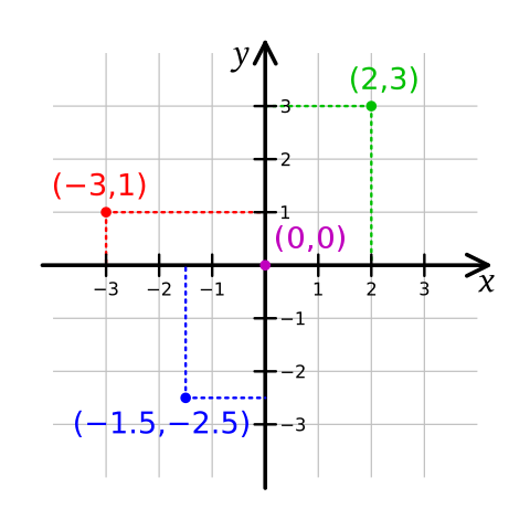
The Cartesian coordinate system is the coordinate system most commonly used, where a point in the plane is identified by its horizontal distance and vertical distance to a reference point called origin. These two values are called coordinates, the horizontal axis is called x-axis, and the vertical one y-axis. See Coordinate system to see the details on how this is implemented in Punctual.

fx, fy, fxy

As explained in fragments, Punctual expressions are evaluated for each fragment. For a given fragment, fx is the x-coordinate of that fragment, fy is the y-coordinate, and fxy is a list with both coordinates.

The next examples are some creative ideas one can explore using only coordinates and basic mathematical functions.

Dividing the screen in 10 vertical gradients:

5 * (fx % 0.2) >> add;

The modulus fx % 0.2 (see mathematical functions for more information) makes 10 stripes from 0 to 0.2 (10 as fx goes from -1 to 1). Then, we multiply by 5 to rescale the value to a 0 to 1 range.

Color patterns

Here we are using three simple formulas to get each of the three RGB channels directly from the coordinates of each fragment.

-- Try changing abs by unipolar
abs [fx, (-1)*fy, (fx+fy)/2] >> add;

unipolar $ (-1)*fx++fxy >> add;

[unipolar $ sin' fx, 1 - abs fy, unipolar $cos fx] >> add;

There are a lot of formulas that allow you to make cool gradients as a starting point for more complex transformations.

See Colors for some ideas on using other colors spaces aside from RGB.

Using punctual to draw mathematical functions:

A typical mathematical function has the form y=f(x), where f(x) is a formula that specifies how to get the y coordinate from the x coordinate. So, for any x, we draw a point at coordinates (x, f(x)).

Using this method we can draw a lot of mathematical functions (here, the zoom is only used to see a bit more of the resulting graph):

zoom 0.4 $ point [fx, cos fx] >> add;

zoom 0.4 $ point [fx, log $ abs fx] >> add;

zoom 0.4 $ point [fx, fx*fx] >> add;

Another way to do the same is by using the between function (see Mathematical functions).

In essence, between receives two values and a graph and returns 1 if the graph is between the two values, or else 0.

Remember that this is evaluated independently for each fragment, so in the next example, for any fragment (fx,fy) we’ll draw white if and only if fy is almost equal to cos fx. The 2*px is the margin that fy can be away from cos y and still be white, and determines the wideness of the line we’ll draw. As explained a bit later, px is the fragment’s height:

zoom 0.4 $ between [cos fx-2*py, cos fx+2*py] $ fy >> add;

We can use evolve these ideas to create interesting patterns:

point[fx, osc 0.09*cos (fx*fy*15*(2+osc 0.32))] >> add;
0.98 * fb fxy >> add;

px, py

Depending on the screen resolution and the windows size, pixels on Punctual will have a specific dimensions expressed in the Punctual coordinate system.

You can access a pixel’s width with px and a pixel’s height with py. This is usually used to draw thin lines, as in the following example, or the ones on the previous section:

zoom 0.4 $ circle [fx, fx*fx] $ 4*px >> add;

aspect, fit

aspect is the ratio between the width and height of the window, so, if you don’t change the window size (or use fit), it’s a constant.

To “see” it’s value, we can try something like this:

[0.3*aspect,0,0] >> add;

Now, change the window size, and you should see how the background is redder as the width height ratio increases, and darker as it decreases.

fit can be used to rescale the x coordinates in order to change the aspect ratio of the result. When doing this, the visible coordinates on the x-axis no longer will be on the range -1 to 1 (unless fit aspect is specified, which is the same as doing nothing).

The most obvious way of using fit is to correct the aspect of geometric shapes, so a circle draws like a circle, and so on:

fit 1 $ circle 0 0.3 >> add;

fit 1 $ rect 0 0.5 >> add;

Another useful application of fit is to scale an external source (an image, a video, or the camera output) to fit the screen, or a particular portion of the screen:

fit (0.5*aspect) $ move [1, 0] $ img "https://upload.wikimedia.org/wikipedia/commons/d/d4/Karl_Marx_001.jpg" >> add;
fit (0.5*aspect) $ move [-1,0] $ img "https://upload.wikimedia.org/wikipedia/commons/2/21/Friedrich_Engels_portrait_%28cropped%29.jpg" >> add;

In this example, we took images of the Communist Manifesto authors from Wikicommons, and made each one of them to occupy the half of the window, independently from its size.

Same idea, but we divide the window in two horizontally:

fit (2*aspect) $ move [0,-1] $ img "https://upload.wikimedia.org/wikipedia/commons/8/87/Tundra_in_Siberia.jpg" >> add;
fit (2*aspect) $ move [0,1] $ img "https://upload.wikimedia.org/wikipedia/commons/2/2d/Picea_glauca_taiga.jpg" >> add;

Can we combine both previous examples to divide the window in four equal-sized parts? The answer is yes, as aspect is modified just when fit is executed:

fit (0.5*aspect) $ fit (2*aspect) $ move [-1,1] $ img "https://upload.wikimedia.org/wikipedia/commons/2/2d/Picea_glauca_taiga.jpg" >> add;

Now, these last examples show the most standard uses of fit, but you can also use it in many creative ways.

For example, we can apply an oscillator to the aspect ratio to deform the image periodically:

fit (osc 0.2) $ circle 0 0.8 >> add;

Now, evolving this example, we can create beautiful patterns:

spin [saw 0.2, (-1)*saw 0.2] $ fit (8*osc (0.5*cps)) $ tile [4,step [1,4,8,16] $ saw cps] $ circle 0 0.8 * [0.8,0,0.8]>> add;
0.8 * fb fxy >> add;

Here, we are synchronizing the fit oscillator to the beat, and increasing its range to -8 to 8. We are also drawing a lot more circles using tile. The replication over the y-axis changes over time, due to the use of step and the saw oscillator. Finally, the spin with to graphs as first argument, duplicates the whole set and made each of the copies rotate in opposite directions.

Polar coordinates

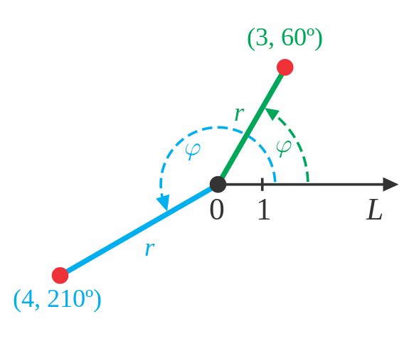
In the polar coordinate system, each point in the plane also has two coordinates, but they are the distance to the pole (the center of the window, analogous to the origin in Cartesian coordinates), and the angle from the horizontal ray that goes from the pole to the right (called polar axis), measured in radians.

fr, ft, frt

In the same way that fx, fy and fxy allow to get fragment coordinates in the Cartesian system, fr, ft and frt are the fragment coordinates in the polar system.

fr is the distance from the pole, and is equivalent to dist 0 or dist [0,0].

Note that if we only move through one of the axis, fr goes from 0 to 1, but can be larger. The point at [1,1] has a fr of approximately 1.41, that is the square root of 2 (by the Pythagorean theorem).

ft is the angle from the reference ray, which is the right part of the horizontal axis. In Punctual, this angle goes from -π to π radians. This is important, as many times you’d like to rescale this range to a [-1,1] range or [0,1] range, in order to use it in other parts of your code:

• To a [-1,1] range: ft/pi.
• To a [0,1] range: linlin [(-1)*pi, pi] [0,1] ft or unipolar $ ft/pi.

Next examples are similar to the ones of the Cartesian coordinates section, but the result can be quite different when using polar coordinates.

20 radial gradients:

fit 1 $ 10/pi*(ft % (pi*0.1)) >> add;

Or concentric gradients:

fit 1 $ 10 * (fr % 0.1) >> add;

Color patterns:

r << fr/1.4;
t << ft/pi;
[1-r, abs t, abs $ r/ft] >> add;

r << fr/1.4;
t << ft/pi;
[1-r, abs t, abs $ fx*fy] >> add;

Note how fr and ft are rescaled to keep the red and green coordinates from 0 to 1.

Mathematical functions:

Not so obvious as with Cartesian coordinates, but it’s possible to build interesting shapes using the same ideas:

fit 1 $ point [fx, sin' ft] >> add;

For each fragment, draw only the points where y matches the sine of the angle. This results in a circumference of radius 1 (by definition of the sine function, the sine of an angle is the y coordinate of the corresponding point on the circumference of radius 1), and a line at x=0, as the sine of 0 (or π) is 0.

The missing central part of the line is due to rounding errors. Actually, point is a small circle, so it’s visible if some fragment is near enough the specified coordinates. That explain why the circumference has some wideness. Now, as we get closer to the origin, a little change in coordinates radically changes the angle, and that’s why there isn’t any point there which sine is near enough to the y coordinate.

Similarly: fit 1 $ between [sin' ft - py, sin' ft + py] $ fy >> add;.

dist, prox

dist is the distance of a fragment to a given position.

prox is the opposite of dist, the idea of proximity of a fragment to a given position. prox is calculate such as two opposite screen points have a proximity of 0, and one point has a proximity of 1 to itself.

Let’s take for example [1,1] and [-1,-1] as two point that are as far away from each other as it is possible in the initial visible screen. The distance between them, per the Pythagorean theorem, is the square root of 8, that is approximately 2.828427. prox is computed as (2.828427-dist[x,y])/2.828427, clamped to be between 0 and 1.

One very usual way of using prox is to create masks. Visuals can get quite bright easily, and this can make it difficult for you or the people you are jamming with to see the code on the screen.

You can create a mask in order to keep the borders of the screen relatively clear and focus the visuals on the center:

a << 1;
m << prox 0 ** 4;
a*:m >> add;

Here, a is the annoying graph, in this case a completely white screen. m is the mask, calculated as the proximity to the origin, and raised to the power of 4.

Note that, as all proximities lies between 0 and 1, as we increase the power, the resulting numbers will be nearer to 0.

Finally, we multiply a and m, point to point, deeming each fragment according to the proximity it has to the center.

Following there are some examples on how can we use dist and prox in different creative ways:

• Color patterns depending on the distance of each fragment to certain coordinates:

[dist [0.5,0], prox [-0.6,-0.3], dist [-0.3,0.3]] >> add;

• Deform an image:

i1 << img "https://upload.wikimedia.org/wikipedia/commons/0/0c/Golden-eyed_tree_frog_%28Agalychnis_annae%29_1.jpg";
tile [prox [0.5,0], 3*dist [0,0.2]] $ i1 >> add;

Here we use tile (see geometric transformations) to deform the image, as the value of tile is different for each fragment.

We can add some audioreactiveness (see audio reactive visuals) to the last pattern to make it a bit more interesting:

i1 << img "https://upload.wikimedia.org/wikipedia/commons/0/0c/Golden-eyed_tree_frog_%28Agalychnis_annae%29_1.jpg";
tile [prox [ihi,0], 3*dist [0,ilo]] $ i1 >> add;

From Cartesian to polar and viceversa

There are a bunch of functions that are meant to transform coordinates from the Cartesian system to the polar system or viceversa:

xyrt: from Cartesian to polar.

To understand this function let’s look at the following example:

c << [1,osc 0.1];
fit 1 $ [circle c 0.1, circle (xyrt c) 0.1] >> add;

The red circle stays at x=1 and moves vertically, from y=-1 to y=1 due to the oscillator.

The cyan circle is very similar, but we’ve applied xyrt to its center coordinates. That means that these coordinates are transformed to polar coordinates. So, looking at the first circle and thinking in how this movement affects the angle and radius from the center, we see that the angle moves from -pi/4 to pi/4, that is from approximately -0.79 to 0.79. The radius moves from the square root of two (1.41) at the top, then decreases until it get to 1, just on the horizontal axis, and then increases again to 1.41 at the bottom.

Now we take these two coordinates, but read them as Cartesian coordinates (note that xyrt calculates the polar coordinates, but doesn’t apply any real geometric transformation like setfxy does). So, the result is a circle which x coordinate moves from 1.41 to 1 then again to 1.41, and which y coordinate moves from -0.79 to 0.79.

Let’s add a few reference lines to check our calculations:

c << [1,osc 0.1];
fit 1 $ [circle c 0.1, circle (xyrt c) 0.1] >> add;
mono $ fit 1 $ hline [-0.79, 0.79] px >> add;
mono $ fit 1 $ vline [1,1.41] px >> add;

As a side note, see how the first example can be rewritten shorter using the ++ operator from the combining graphs section:

c << [1,osc 0.1];
fit 1 $ circle (c++xyrt c) 0.1 >> add;

xyr, xyt

These two functions are nearly identical to xyrt, but they only return one of the two coordinates, the radius or the angle respectively.

Following the previous example:

c << [1,osc 0.1];
fit 1 $ [circle c 0.1, circle [xyr c,0] 0.1] >> add;
mono $ fit 1 $ vline [1,1.41] px >> add;

c << [1,osc 0.1];
fit 1 $ [circle c 0.1, circle [0,xyt c] 0.1] >> add;
mono $ fit 1 $ hline [-0.79, 0.79] px >> add;

rtxy: from polar to Cartesian.

This is the opposite from xyrt: it takes coordinates in the polar system and returns the equivalent in the Cartesian system.

c << [1,pi*osc 0.1];
fit 1 $ zoom 0.25 $ circle (c++rtxy c) 0.1 >> add;

The red circle keeps its x coordinate at 1 and oscillates between -π and π on the y coordinate (note the zoom in order to see all its movement).

The cyan circle takes the 1 as its distance from the origin, and changes the angle, so it keeps moving around the origin, always at the same distance.

I find that rtxy is the most usable of the whole family to create cool visual effects.

In the next example, let’s start with this:

c << [[0.2,0.3..2]*:osc 0.12*osc 0.13, pi*osc 0.1*osc 0.11];
zoom 0.25 $ circle c 0.1 >> add;

These are a bunch of circles that move together in a somewhat irregular way due to the multiplications of oscillators at different frequencies.

The first bit ([0.2,0.3..2]) uses Haskell style list expansion to create the x coordinate for each circle, from 0.2 to 2, going in steps of 0.1.

The y coordinate is common to all circles, and oscillates from -π to π.

Next step is just take all the circle’s center coordinates and read them as polar coordinates.

c << [[0.2,0.3..2]*:osc 0.12*osc 0.13, pi*osc 0.1*osc 0.11];
circle (rtxy c) 0.1 >> add;

Now, we apply some basic geometric transformations, using combinations of fx, fy, ft and fr to twist the circles geometry:

c << [[0.2,0.3..2]*:osc 0.12*osc 0.13, pi*osc 0.1*osc 0.11];
fit 1 $ spin (fr*4) $ move [ft*fx*0.3,ft*0.1] $ circle (rtxy c) 0.1 >> add;

Finally, let’s add some repetition in the middle to create more elements:

c << [[0.2,0.3..2]*:osc 0.12*osc 0.13, pi*osc 0.1*osc 0.11];
fit 1 $ spin (fr*4) $ tile [4,4] $ move [ft*fx*0.3,ft*0.1] $ circle (rtxy c) 0.1 >> add;

Playing with circles and polar coordinates is fun! In the last example, all the circles were moving like a whole. Can we make each one to move separately from the others?

Let’s start with our circles forming a bigger circumference around the center:

t << linlin [0,1] [0, 2*pi] [0, 0.02..1];
fit 1 $ circle (rtxy [0.5, t]) 0.1 >> add;

Here we use a list expansion for the circles angles, just like in the last example, and rescale it from a 0 to 1 range to a 0 to 2π using linlin, just because it’s easier to think from 0 to 1.

Then draw all the circles using polar coordinates, at a fixed distance from the origin of 0.5.

Let’s made the circles spin:

t << linlin [0,1] [0, 2*pi] [0, 0.02..1];
o << pi * saw 0.1;
fit 1 $ circle (rtxy [0.5, t+:o]) 0.1 >> add;

Here, o is an oscillator that goes from -π to π, and when it reaches π it starts again from -π. We add this oscillator to each angle, and the result is that all the circles spin together.

Finally, let’s apply an oscillator to the radius too, but this time, each circle will have a distinct frequency, so they will move apart from each other. We make this by using t to modify the oscillator frequency in the bit osc (0.1*t).

Now, we have a list of radius and a list of angles, and we need to link them together: the first radius with the first angle, the second radius with the second angle, and so on. This is just what the zip function from combining lists does.

As a final touch, we use mono to combine all channels into one, which make all circles white:

t << linlin [0,1] [0, 2*pi] [0, 0.02..1];
o << pi * saw 0.1;
fit 1 $ mono $ circle (rtxy $ zip (osc (0.1*t)) (t+:o)) 0.1 >> add;

rtx, rty

These two functions are nearly identical to rtxy, but they only return one of the two coordinates, the x or y coordinate respectively.

r << unipolar $ osc 0.03;
t << pi*osc 0.07;
fit 1 $ circle [r,t] 0.1 >> add;
fit 1 $ circle (rtxy [r,t]) 0.1 >> red;
fit 1 $ circle [rtx [r,t], 0] 0.1 >> green;
fit 1 $ circle [0, rty [r,t]] 0.1 >> blue;

In this example, r oscillates from 0 to 1, and t from -π to π. There are a total of four circles:

• White: r and t are interpreted as Cartesian coordinates x and y.
• Red: r and t are read as polar coordinates.
• Green: r and t are polar coordinates, but only used to calculate the resulting x position.
• Blue: same as green, but only the y position is calculated.

Examples

10 ways of drawing a circumference of radius 1

Just to see the flexibility of Punctual and different ways to use coordinates, let’s think of different ways to draw a circumference of radius 1.

Probably the easiest way: let’s paint white (1) all fragments whose radius is 1, pixel more, pixel less:

between [1-px, 1+px] $ fr >> add;

As the radius is no more than the distance to the origin, this is equivalent:

between [1-px, 1+px] $ dist 0 >> add;

Also, it’s possible to make this calculation explicit, using the Pythagorean theorem:

between [1-px, 1+px] $ sqrt $ fx*fx+fy*fy >> add;

Next is a similar approach, but without using between. Here, on one hand we take all fragments whose radius is a bit lesser than one, and on the other the fragments whose radius is a bit greater than one. What we want is the intersection of those two, so we multiply the graphs (the result will be one only if both graphs have a one on that fragment).

(fr <= 1+px) * (fr >= 1-px) >> add;

Another way of thinking this is by using the mathematical function of a circumference. For any x, we have to paint only the y that follow the formula x^2 + y^2 = 1. Isolating the y we get:

f << [-1,1]*(sqrt $ 1-fx*fx);
mono $ point [fx, f] >> add;

Note how the square root is multiplied by [-1,1] in order to take both roots.

Now we can take both ways of thinking and mix them. We’ll paint white only those fragments whose x-coordinate is near the computed y for the circle at that x:

c << sqrt (1-fy*fy);
between [c-px, c+px] $ abs fx >> add;

In the last example, we are only taking the positive root of the square root, but are taking the absolute value of x to make the graphic symmetrical.

Yet another way of thinking this problem: we already have a function that draws circles. Let’s tweak it to draw a circumference instead.

In this example, we draw a circle of radius 1, and then take off a slightly smaller circle:

(circle 0 2) - (circle 0 $ 2-2*px) >> add;

Next is mathematically equivalent to the last one, but we get here with another way of thinking. We can draw the inner part of the circumference with a circle, and also the outer part with an inverted slightly bigger circle (using 1- to invert the result, as it is all 0 and 1). So, we have obtained just the invert of what we what, so we invert the result again:

1-(1-circle 0 (2+2*px) + circle 0 (2-2*px)) >> add;

Finally, a last way to solve the problem is by transforming coordinates from Cartesian to polar. If you think about it, a circumference has a very easy representation on polar coordinates, as one of them (the radius) is constant.

This is exactly what vertical and horizontal lines are: a graph where one of the two coordinates is constant.

So we can draw a vertical line, and then think of it a circumference in polar coordinates, so when we interpret the x as the radius and the y as the angle, we get a circumference:

setfxy frt $ vline 1 px >> add;

Similarly, we can use a horizontal line, and the we need to interpret the x coordinate as the angle, and the y coordinate as the radius:

setfxy [ft,fr] $ hline 1 px >> add;

Bonus track: set feedback to 100% and use a point like it is a pencil:

spin (saw 0.06) $ point [0,1] >> add;
fb fxy >> add;

Implementing Hydra functions

As explained in the Overview, Hydra is a popular language for live-coding visuals. One key difference between Hydra and Punctual is that Punctual operates at a slightly lower level than Hydra.

This means that while it is possible (though not always straightforward) to reimplement many Hydra functions using Punctual, the reverse is not necessarily true.

Let’s develop a couple of examples to illustrate this.

• Implementing Hydra’s osc() function:

Hydra’s osc() function draws a sine wave, visualized from above. When the sine wave is far away (low), the visualization appears black, and as it gets closer, it turns white.

In Punctual, this can be expressed using unipolar $ sin' (fx*freq), where freq determines the number of sine wave repetitions. To fully mimic Hydra’s osc(), we need to adjust the coordinates and use unipolar fx instead of fx: unipolar $ sin' (unipolar fx*freq).

Hydra’s osc() also moves horizontally over time. We can achieve this by adjusting the phase of the sine wave based on the elapsed time:

unipolar $ sin' ((unipolar fx+sync*time)*freq);

Hydra uses 60 as the default frequency and 0.1 for the sync parameter. Applying these values, the Punctual expression becomes:

unipolar $ sin' ((unipolar fx+0.1*time)*60) >> add;

This expression recreates the behavior of Hydra’s osc() function in Punctual.

• Implementing osc().kaleid():

Now that we have our version of Hydra’s osc() function, we can extend it with some transformations, such as kaleid().

In this example, we are reimplementing the Hydra expression osc().kaleid(5).out().

The core idea of kaleid(5) is to apply a geometric transformation (using setfxy) by which we take an arc of a fifth of the whole circle and copy it five times, filling the entire screen. Additionally, we need to rotate our arc so that the different parts align correctly, and apply a translation because Hydra’s kaleid() copies the upper left part of the image but draws it at the center.

This is a possible implementation:

hosc << unipolar $ sin' ((unipolar fx+0.1*time)*60);
k << ft % (2*pi/5);
setfxy (rtxy [fr, k]) $ spin ((-1)/5) $ move 0.5 hosc >> add;

1. First line: This is our version of Hydra’s oscillator, osc(), which creates a sine wave pattern that moves horizontally over time.
2. Second line: Here, k is defined. It represents the new angle for each fragment, and the modulus (%) operator is used to map any fragment to the first fifth of the circle. This is the key to the whole kaleidoscope effect.
3. Third line: This line combines several transformations:
   • move 0.5 hosc: Moves the oscillator 0.5 units in each coordinate, effectively shifting the top-left corner of the screen to the center.
   • spin ((-1)/5): Rotates one-fifth of the whole circle, ensuring that each part of the pattern matches up seamlessly.
   • setfxy (rtxy [fr, k]): Applies the geometric transformation. Note that setfxy (rtxy frt) something is an identity transformation, as it retains the radius and the angle. In our cas, k is assigned as the new angle, effectively creating the kaleidoscope effect by repeating and rotating the pattern.

This implementation effectively mimics Hydra’s osc().kaleid(5).out() by using Punctual’s lower-level functions to achieve the same visual result.

setfxy is so flexible that we could include the move, spin and rtxy operations inside the setfxy transformation making the whole transformation in only one step:

hosc << unipolar $ sin' ((unipolar fx+0.1*time)*60);
k << ft % (2*pi/5)-pi/5;
setfxy (fr*[cos k, sin k]-0.5) hosc >> add;

Of course, this is complicated to deduce, but as Hydra is free software, we can look up the original kaleid implementation and translate the code to Punctual.