Combining graphs

In this section, some of the operators used to combine graphs are studied.

One of Punctual’s important characteristics is that it’s combinatorial by default. This means that usual arithmetics operators like + or * are combinatorial, and there exist another whole set of operators which are pairwise (+: and *: instead of + and *).

Combinatorial binary operators

A combinatorial operator create all possibilities that result from combining any channel from the first graph with any channel from the second graph.

For example, [0.1, -0.1] + [0.3, 0.2] results in the expression [0.4, 0.3, 0.2, 0.1], and [0.1, 0.2, 0.3] + [0.3, 0.6] is [0.4, 0.7, 0.5, 0.8, 0.6, 0.9].

The list of combinatorial binary operators is as follows:

• Arithmetic:
  • +: addition, 8+2=10
  • -: subtraction, 8-2=6
  • *: multiplication, 8*2=16
  • /: safe division. Like usual division, but the result of dividing anything by 0 is 0. 8/2=4
  • **: exponentiation, 8**2=64.
  • %: modulo. The remainder obtained after dividing the first argument by the second. 8%2=0, 8%3=2.
• Comparison: these operators return 1 if the condition is met and 0 if not.
  • ==: equal to. 8==2=0, 8==8=1
  • /=: not equal to. 8/=2=1, 8/=8=0
  • >: greater than. 8>2=1, 2>8=0, 8>8=0
  • >=: greater than or equal. 8>=2=1, 2>=8=0, 8>=8=1
  • <: less than. 8<2=0, 2<8=1, 8<8=0
  • <=: less than or equal. 8<=2=0, 2<=8=1, 8<=8=1

Let’s start with a very simple example just to see how graphs are combined:

p << [0.1,-0.1]+[0.3,0.2];
--p << [0.4,0.3,0.2,0.1];
circle p 0.1 >> add;

Note that the first and second (commented out) lines are equivalent.

In the next example, a complex pattern of points is created, using list expansions and the combinatorial operators + and *.

There are 7 channels in the first list and 5 channels in the second. That results in p having 35 channels. o has 11 more channels, so p2 has a total of 35*11=385 channels. Now, the center of a circle has two coordinates, so there are 193 circles (the last, odd one duplicates its only coordinate).

We don’t really want so many channels, only a lot of circles, so we add mono to convert the signal to a 1-channel expression, and then apply some color. Note that there are some circles that have a stronger color than others. That is because there are circle that always have the same coordinates as a result of the combination of all possibilities between the first and second lists (we can force the separation of these circles by using different numbers in one of the lists; for example, try to replace the second list by [0.33,0.21,0.02,-0.18,-0.49]).

p << [0.3,0.2..(-0.3)]+[0.3,0.2,0,-0.1,-0.4];
o << osc [0.05,0.04..(-0.05)];
p2 << p * o;
(mono $ fit 1 $ circle p2 0.03) * [fr, 0, 2*fr] >> add;

In the following example, we use the channel separation functions from colors to move only some fragments from the original image. Here, the expression rgbb i>rgbr i returns 1 only for the fragments where the blue component is greater than the red component. Then, those fragments are slowly displaced up (faster as the blue component is higher). The result is an interesting effect where the smoke in the image moves, but the fire don’t.

i << tile [3,1] $ img "https://upload.wikimedia.org/wikipedia/commons/thumb/c/c1/Streichholz.jpg/400px-Streichholz.jpg";
move [0,(unipolar $ saw 0.08)*rgbb i *(rgbb i>rgbr i)] $ i >> add;

Pairwise binary operators

A pairwise operator joins two expressions by combining channels by pairs: the first channel of the first operand with the first channel of the second operand, and so on: [1,3,5] +: [3,4,5] is equivalent to [4,7,10].

When one of the operands has less channels than the other, the shorter one is cycled: [1,3,5] +: [3,4] is equivalent to [4,7,8].

Note that when one of the two operands has only one channel, using a combinatorial or a pairwise operator yields the same result.

The list of pairwise binary operators is as follows:

• Arithmetic: +:, -:, *:, /:, **:, and %:.
• Comparison: ==:, /=:, >:, >=:, <:, and <=:.

Note the difference between the next two expressions:

point [fx, osc [0.03, 0.04, 0.05] * sin' fx + [0.2,-0.2]] >> add;

point [fx, osc [0.03, 0.04, 0.05] * sin' fx +: [0.2,-0.2]] >> add;

In the first one, the + is combinatorial, so each oscillator is duplicated, and the result is six sinusoidal curves that move grouped in three pairs.

In the second example, where +: is used, the addition is pairwise: 0.2 is added to the first (red) curve, -0.2 is added to the second (green) curve, and, as there are no more numbers in the second list, the first 0.2 is taken again and added to the third (blue) curve.

The next example presents a simple level meter. As the sound captured by the mic is louder, more circles appear:

l << [0, 0.1 .. 0.9];
a << imid > l;
c << circle [0, l-0.2] 0.1;
fit 1 $ mono $ c *: a >> add;

l has 10 channels. a combines a 1-channel expression (imid) with l, so it also has 10 channels. a has only a 0 or a 1 in each channel, depending on if the middle frequencies amplitude is higher than each of the thresholds in l (see audio-reactive visuals).

Then, c contains a total of 10 circles, all at the same x coordinate but different high. When multiplying c by a, only the circle that are paired with a 1 will be visible.

Next, we recreate the Savamala logo in Punctual:

bg << fx<=fy;
x1 << [0.2,0.2,0.5];
x2 << [0.8,0.5,0.8];
y1 << [-0.2,-0.2,-0.8];
y2 << [-0.2,-0.8,-0.2];
t1 << mono $ line (zip x1 y1) (zip x2 y2) 0.05;
t2 << mono $ line (zip (x1-1) (y1+1)) (zip (x2-1) (y2+1)) 0.05;
fit 1 (bg+:t1-:t2) >> add;

Note how the background is built using the <= operator on the first line. Then, we write down the coordinates of one of the triangles: x1 and y1 contain the starting points of the three lines, and x2 and y2 the ending points. We use zip to put together each x coordinate with its corresponding y coordinate. t2 is built by modifying t1 coordinates; note how -1 and +1 affects the whole list. Finally, we use +: and -: to add the first triangle to the background (white over black) and subtract the second triangle (black over white).

o << saw 0.5;
p << [0.8*o+(8*(o>=0.9)),0.3];
c << hsvrgb [unipolar $ osc 5.13,0.8,1];
l << circle p 0.05;
l*c >> blend;
move [0,(-0.025)*(o>0.9)] $ fb fxy >> add;

0.3 >> add;
hline 0 (1/6*aspect) >> blend;
hline ((-1)/3*aspect) (1/6*aspect) * [0,0.59,0.21,1] >> blend;
hline (1/3*aspect) (1/6*aspect) * [0,0,0,1] >> blend;
m1 << (-0.75)*aspect; b1 << (-0.25)*aspect;
l1 << m1*fx+b1 > fy;
m2 << 0.75*aspect; b2 << 0.25*aspect;
l2 << m2*fx+b2 < fy;
l1*l2 * [0.93,0.16,0.21,1] >> blend;

Combinatorial binary functions

min, max, gate

In addition to the multiple operators, there are several functions, min, max and gate, that also combine two graphs in a combinatorial way.

As the name implies, min combines each pair of elements by selecting only the smallest, and max by taking the biggest.

Don’t forget that they are combinatorial, so elements in each graph are combined in all possible combinations:

ys << min [0.1,0.5,0.3] [0.4,0.2,0.6];
hline ys 0.01 >> add;
--hline [0.1, 0.1, 0.1, 0.4, 0.2, 0.5, 0.3, 0.2, 0.3] 0.01 >> add;

Here, the third line is equivalent to the first two lines. From the bottom to the top, the first white line results from the first three 0.1. The green line is the combination of the two 0.2 (note that both are interpreted as green, as they are in the second channel of a group of three). The purple line is the result of combining the two 0.3, which are red and blue. The red line is the 0.4 on the forth position, and the blue line is the 0.5 on the sixth position.

One possible creative use of min and max is combining two images or videos. In the next example, the same video is combined with itself, but on each copy, a color transformation is applied:

v << vid "https://upload.wikimedia.org/wikipedia/commons/1/1b/Rundflug_um_den_Perchtoldsdorfer_Wehrturm.webm";
min (rgbhsv v) (hsvrgb v) >> add;

v << vid "https://upload.wikimedia.org/wikipedia/commons/1/1b/Rundflug_um_den_Perchtoldsdorfer_Wehrturm.webm";
0.5*max (rgbhsv v) (hsvrgb v) >> add;

Note that min and max are combinatorial, so the above examples result in 9-channels signals. This explains why the results are so bright, even when using min.

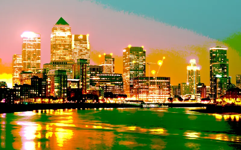
gate [graph] [graph]: The first graph acts as a limiter to the second; on fragments where the first graph is greater than the second, the result is 0. Otherwise, the result is the value of the second graph. For example, gate 0.3 0.4 result in 0.4, gate 0.4 0.3 results in 0, gate fx fy result in 0 below the diagonal defined by fx=fy, and fy above it.

In the next example, a gate is applied to a city image. The gate gradually closes, and as it does, more and more fragments turn black. The overall result resembles the sunset in the city.

Note how the gate is applied to each color component independently.

i << img "https://upload.wikimedia.org/wikipedia/commons/c/c5/Canary_Wharf_from_Limehouse_London_June_2016_HDR.jpg";
gate [unipolar $ saw 0.06] i >> add;

The next example comes with three variations. You can test each of the commented-out lines to see the results.

It demonstrates the use of gate with a multi-channel graph. In the first variation, gate produces a 6-channel signal (2 channels from the first graph multiplied by 3 channels of the second). Then, unrep is used to join the channels in groups of 2, resulting in a 3-channel signal suitable for the rgb output. The combination of gate and unrep modifies and then mixes the original image colors.

In the second variation, gate produces a 9 channel signal, so we use unrep 3 to get the desired 3-channel result.

For comparison, in the third variation, the pairwise version of gate, gatep, is used. This applies a 0.3 gate to the image’s red channel, a 0.6 gate to the green one, and 0.2 to the blue one, keeping the same 3 channels as the original image.

i << img "https://upload.wikimedia.org/wikipedia/commons/c/c5/Canary_Wharf_from_Limehouse_London_June_2016_HDR.jpg";
unrep 2 $ gate [0.3,0.6] i >> add;
--unrep 3 $ gate [0.3,0.6,0.2] i >> add;
--gatep [0.3,0.6,0.2] i >> add;

Other combining operators

++

• ++: joins two graphs by appending the second one after the first one. The resulting graph has as many channels as the sum of the channels in the two original graphs. For example, [1,2,3]++[4,5] is [1,2,3,4,5].

We have already used this operator to combine lists and to add an alpha channel to RGB colors (for example, in Color spaces translation). However, it can be used to combine any graphs in different channels.

In this example, we start with a rectangle and apply several different transformations to it, resulting in three different shapes r1, r2 and r3. Then, we combine all three shapes with ++. Note how r3 is mapped to the red channel, r2 to the green one, and r1 to the blue one:

o << 0.1~~0.5 $ tri 0.12;
r1 << move (0.5*(fy%o)) $ rect 0 0.8;
r2 << spin (abs fx) r1;
r3 << spin (fr+saw 0.15) $ zoom (0.8+2/3*abs fx) r1;
r3++r2++r1 >> add;

[[]]

• [[]]: when there is a list inside another list, Punctual expands them in a combinatorial way. For example, [1,[2,3],4,5] is equivalent to [1,2,4,5,1,3,4,5].

In this example, we take advantage of this property to build a long list for the step function, creating variation inside the repetition.

l represents a mirrored vertical line that moves at the speed defined by s. s is used again to define the variation in the red component of the line’s color, and a third time to determine the speed at which the feedback will rotate.

The result is a succession of geometric patterns that transition smoothly from one to the next.

s << step [[-0.1,0.1],0.02,0.04,-0.03] $ saw 0.03;
l << mono $ setfx [fx, (-1)*fx] $ vline (0.5*osc s) 0.002;
co << [unipolar $ osc s,0,0.7,0.8];
l*co >> blend;
gatep 0.2 $ spin s $ 0.99*fb fxy >> add;

Pairwise binary functions

maxp, minp, gatep

• maxp, minp, gatep: these functions are the pairwise equivalents to max, min and gate seen before.

Let’s rewrite the min and max examples using minp and maxp to compare the results:

v << vid "https://upload.wikimedia.org/wikipedia/commons/1/1b/Rundflug_um_den_Perchtoldsdorfer_Wehrturm.webm";
minp (rgbhsv v) (hsvrgb v) >> add;

v << vid "https://upload.wikimedia.org/wikipedia/commons/1/1b/Rundflug_um_den_Perchtoldsdorfer_Wehrturm.webm";
maxp (rgbhsv v) (hsvrgb v) >> add;

The resulting colors are quite different this time, and the overall brightness is similar to the original video, as we are combining two 3-channel signals to get another 3-channel signal.

In the following example, gatep is employed to remove each color component based on the fragment coordinates. The red component is eliminated at the right and left edges of the screen. The green component is removed along the y-axis. The blue component is removed depending on the angle; it is retained in the bottom-left part and gradually removed as we rotate counterclockwise:

v << vid "https://upload.wikimedia.org/wikipedia/commons/1/1b/Rundflug_um_den_Perchtoldsdorfer_Wehrturm.webm";
gatep [abs fx,unipolar fy,linlin [(-1)*pi,pi] [0,1] ft] v >> add;