Color in Punctual is intimately related to channels.
Colors and output notations
Depending on the output notation used, channels are interpreted as colors in different ways (see output notations):
add,rgb,mul: first channel is red, second green, and third blue. If there is less than 3 channels, they are read following these rules:- One channel: the same value is used for the three base colors, resulting in a gray level, from 0 black to 1 white.
- Two channels: the first channel is red, the second is used for both blue and green, resulting in cyan.
- More than three channels: every 3 channels are a group of red, green, blue, any excess is read as in the previous rules. So, for example, a 5-channel signal would be red-green-blue-red-cyan, and a 4-channel signal red-green-blue-white.
blend,rgba: first channel is red, second green, third blue, and forth is alpha (transparency). Chanel matching works in the same way asadd, but with four output channels, and can be confusing. For example,circle [0,0,0.1,0.1] 0.1 >> blend;is a 2-channel signal. The first circle is red, but it will have 0 on the alpha channel, so it’s invisible. The second circle is cyan and visible, asg,bandaare joined. Therefore, usingblendwith an arbitrary number of channels won’t produce many interesting results.
Basic usage
Most of the times, we’ll create a 1-channel signal and then convert it into a 3-channel signal to get color in the RGB color space. To do this, we only need to multiply our signal by a three elements list. Due to Punctual’s combinatorial nature, our signal will be split in three channels, being the same on all of them, except for the multiplying factor on each one:
circle 0 0.2 * [0.8,0,0.8] >> add;
Note that each color component receives a value from 0 to 1. There is no problem in sending lower or higher values, but they will always be trimmed to this range.
The following table shows the codes corresponding to some basic colors in both the RGB and HSV color-spaces:
| Name | RGB | HSV |
|---|---|---|
| Black | 0,0,0 | 0,0,0 |
| White | 1,1,1 | 0,0,1 |
| Red | 1,0,0 | 0,1,1 |
| Lime | 0,1,0 | 0.33,1,1 |
| Blue | 0,0,1 | 0.67,1,1 |
| Yellow | 1,1,0 | 0.17,1,1 |
| Cyan | 0,1,1 | 0.5,1,1 |
| Magenta | 1,0,1 | 0.83,1,1 |
| Silver | 0.75,0.75,0.75 | 0,0,0.75 |
| Gray | 0.5,0.5,0.5 | 0,0,0.5 |
| Maroon | 0.5,0,0 | 0,1,0.5 |
| Olive | 0.5,0.5,0 | 0.17,1,0.5 |
| Green | 0,0.5,0 | 0.33,1,0.5 |
| Purple | 0.5,0,0.5 | 0.83,1,0.5 |
| Teal | 0,0.5,0.5 | 0.5,1,0.5 |
| Navy | 0,0,0.5 | 0.67,1,0.5 |
| Orange | 1,0.65,0 | 0.11,1,1 |
| Turquoise | 0.25,0.88,0.82 | 0.48,0.71,0.88 |
| Violet | 0.93,0.51,0.93 | 0.83,0.45,0.93 |
| Pink | 1,0.75,0.8 | 0.97,0.25,1 |
| Lavender | 0.9,0.9,0.98 | 0.67,0.08,0.98 |
Of course, things get interesting when we use non constant expressions for the color channels.
Color changes by space
Creating color patterns involves playing with coordinates (fx, fy, fr, ft) and mathematical operations (abs, unipolar, %, and trigonometric functions are pretty useful for this).
There are plenty examples of this on the sections dedicated to Cartesian coordinates and polar coordinates.
color << [abs fx, unipolar fy, fr]/8;
(mono $ fit 1 $ spin (saw [0.03, -0.03]) $ tilex 15 $ vline 0 0.06) * color >> add;
0.95 * fb >> add;
- Red component is defined as
abs fx, so it’s higher on the right and left sides. - Green component is defined as
unipolar fy, so it’s 0 at bottom and 1 at the top of the window. - Blue component is
frso it get higher as we got far from the center. - Note the use of
mono. The signal (before color is applied) it’s a 2-channel signal, due to the list inspin, so when multiplied by the 3-channel color, it would result in a 6-channel signal. The use ofmonoconverts the 2-channel signal into a 1-channel, so it get lighter on the CPU, even though the visual result is the same. - Also note the use of parenthesis to make sure color is applied after the rest of the expression is evaluated. Otherwise, it will only affect the
vlinebit. Withmonothis would result in only white lines (as the 3-channel color would be squashed into a 1-channel signal). Withoutmono, the pattern is completely different, as the color is first applied to the vertical line, and then the other transformations take place.
Color changes by time
There are several ways to make a color pattern evolve through time. One of the easiest is using oscillators (osc, tri or saw), but remember that by default oscillators go from -1 to 1, and a color component from 0 to 1, so many times you will be using unipolar or abs to rescale the values. The ~~ operator is also useful when you don’t want a component to reach all values from 0 to 1 (for example, 0.5 ~~ 0.8 $ osc 0.1 will oscillate only between 0.5 and 0.8).
When using oscillators, you can use a frequency that depends on cps to synchronize the oscillator to the beat (see audio-reactive visuals).
[unipolar $ osc (cps/2), 0.5*abs (tri (cps/4)), 0.3 ~~ 1 $ saw (cps/6)] >> add;
saw is useful to make a flash at each beat. Supposing a 4/4 beat, unipolar $ saw (cps*4) will start at 0 at the beat’s start and end at 1 just when the next beat hits. You can use 1 - unipolar $ saw (cps*4) or the equivalent expression 1-4*(beat%0.25) to make the flash start at 1 with the beat and then fade out. The example is slowed down to reduce the flickering:
slow 4 $ [1-beat%1, 1-4*(beat%0.25), 0] >> add;
You can use late and early to change the phase of an oscillator (see Time shifting functions):
[osc cps, 0, late (cps/2) $ osc cps] >> add;
Note that we haven’t used unipolar here, so really both oscillators are going all the way to -1. We can take advantage of this:
fit 1 $ (1-fr)*:[osc cps, 0, late (cps/2) $ osc cps] >> add;
Color mixing
Any light based device uses an additive color mixing. When two lights are mixed, the frequencies of both are visible, resulting in a clearer color. If enough frequencies are added, the result is white.
In contrast, when using pigments, color mixing is subtractive. Each pigment captures certain light frequencies and reflects the rest. As we add more pigments, more frequencies are captures, and the color is darker, leading to black if we mixed enough pigments.
So by default, Punctual uses an additive color mixing:
iline [-1,1,-1,0,-1,-1] [0,0] 0.2 >> add;
This graph has 3 channels, so the first line is red, the second line is green, and the third one is blue.
Note how colors are mixed together when the lines intersect. For example, when the red and green line intersect the resulting color is yellow ((1,0,0)+(0,1,0)=(1,1,0)). At the center, where the three lines come together, the resulting color is white ((1,0,0)+(0,1,0)+(0,0,1)=(1,1,1)).
An additive color mixing system is prone to end up with a white screen when there are many elements interacting, especially when using feedback.
There are a few tricks we can use to avoid this and still be able to have a lot of different elements interacting.
- Using subtractive color mixing.
Although our computer uses light to show us information and so it’s a naturally additive device, we can simulate a subtractive system by using some calculations.
First of all, let’s say that talking here about subtractive color models is a language abuse. This is a very complex problem that involves the chemical and physical properties of pigments and materials, and are impossible to recreate in a live-coding context.
Fortunately, we don’t need realism. We are just looking for some simple enough calculation we can apply when mixing color that make sure the result won’t be white when things get messy.
Also, we can’t change how colors are automatically mixed when using patterns like the three lines example above. But we can control how colors are mixed when creating patterns, and this by itself it’s quite useful.
Let’s take a very simple approach and say that we mix two colors, c1=(r1,g1,b1), c2=(r2,g2,b2), in a subtractive way by this formula:
c3=(1-abs(r1-r2), 1-abs(g1-g2), 1-abs(b1-b2))
This simple formula works well for basic colors: magenta and yellow will result in red, magenta and cyan will give blue and so on.
In Punctual, we can write the above formula by the very simple expression:
c3 << 1 - (abs $ c1-:c2)
Note how the -: operator takes care of all components at once. Also, avoid using -, because due to the combinatorial nature of this operator you will end up with, you guessed it, white.
Now we can play with complex color patterns and never end up with a white screen:
c1 << unipolar $ osc [0.07, 0.11, 0.06];
c2 << unipolar $ osc [0.05, 0.09, 0.1];
1-:(abs $ c1 -: c2) >> add;
This is just an example formula, we can take other simple ideas (absolutely non-realistic, but our aim is another one): abs $ c1 -: c2, c1*:c2 and so on…
Let’s create a more extreme example. In this case, abs $ c1 -: c2 is used, as it renders darker colors:
a << spin (saw 0.02) $ tilexy [8,4] $ unipolar (spin (saw 0.13) fx);
b << spin ((-1)*saw 0.03) $ tilexy [16,8] $ unipolar $ (spin (saw 0.15) $  fx*fy);
c1 << a*:[unipolar $ osc 0.1,0,unipolar $ osc 0.15];
c2 << b*:[unipolar $ osc 0.3,unipolar $ osc 0.5,0];
c3 << abs $ c2 -: c1;
abs $ c3 -: (spin (saw 0.05) $ zoom 2 fb) >> add;
There a lot of code here, but note that basically, a and b are two patterns of numbers (only one channel per fragment) that depend on fx and fy and spin as time passes.
c1 and c2 are the product of a and b with an oscillating color. If we visualize c1 or c2 by themselves, the pattern is quite simple.
Now, c3 is the mixing of c1 and c2. If we display c3, the mixing of the other two patterns is obvious, but we can clearly see the different colors, as the screen never collapses to white.
Finally, we use feedback to take the last frame, apply some transformations to it, and remix it with c3. The resulting pattern is quite complex, but again, it never gets too bright.
- Using transparency.
One simple way to keep things under control, especially when using high amounts of feedback, is to apply some transparency to your patterns.
Note the difference between these two examples:
0.99 * fb >> add;
co << [abs fx, unipolar fy, fr];
s << slow 10 $ seq [0,0.2,0.4,0.7];
z << (xyrt $ (2+fr)*(abs $ 1-fx)*fy);
sp << [osc 0.035*saw 0.3, (-1)*osc 0.026*saw 0.03];
(mono $ fit 1 $ spin s $ zoomxy z $ spin sp $ tilex 15 $ vline (fy*0.5) 0.06) * co >> add;
0.99 * fb >> add;
co << [abs fx, unipolar fy, fr, 0.8];
s << slow 10 $ seq [0,0.2,0.4,0.7];
z << (xyrt $ (2+fr)*(abs $ 1-fx)*fy);
sp << [osc 0.035*saw 0.3, (-1)*osc 0.026*saw 0.03];
(mono $ fit 1 $ spin s $ zoomxy z $ spin sp $ tilex 15 $ vline (fy*0.5) 0.06) * co >> blend;
Both are the same being the only difference that in the second one we set a 0.5 value to the alpha channel.
In the first example, the screen gets practically white, with some cyan and magenta artifacts forming a vertical and an horizontal line respectively.
In the second example, we can clearly see the patterns that the moving lines are creating, and the screen never gets too bright, even with the high amount of feedback applied.
Note that the order of the operations is important. We need to use blend after add, as seen in Output Notations.
- Gradients.
c1 << [1,0,0];
c2 << [1,0,1];
x << unipolar fx;
c2*x +: c1*(1-x) >> add;
Color spaces
You can use two color spaces in Puntual: RGB and HSV. So far, we’ve been using the RGB color space.
HSV color space is best understood as a mixing of paints. Informally, the hue value represents which color we choose, saturation is the amount of pigment of the chosen color we add, and value is the amount of white light we project on our object.
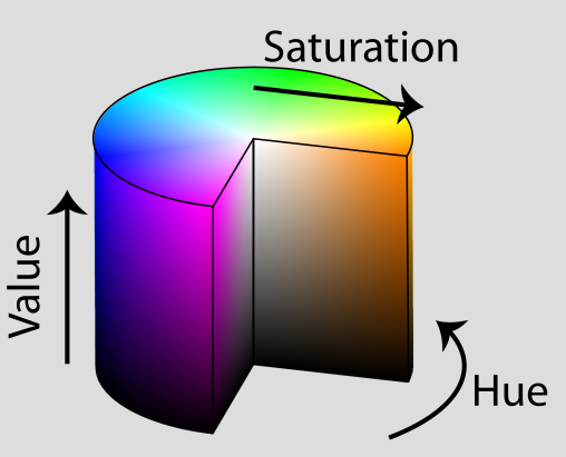
HSV Color space
Jacob Rus, CC BY-SA 3.0, via Wikimedia Commons (edited)
So, for example, if we fix 0.8 (purple) as the hue, and 0.5 as the value, with 0 saturation we get a medium gray and, as we add more and more saturation, the amount of purple increases. Now, if we start to change the value, we can pass from a completely black color with 0, to a very bright purple when we get to 1.
Punctual has functions to isolate one of the channels, translate from one color space to the other, and the combination of these two operations.
rgbr, rgbg, rgbb
rgbr,rgbg,rgbb: use these functions to isolate one of the three channels in an RGB expression. If the input signal has more channels, the result is one channel out of three.
In the next example, we take the red channel of a first video, and the green channel of a second one, then we combine them:
v1 << rgbr $ vid "https://upload.wikimedia.org/wikipedia/commons/4/4f/Midway_Atoll_-_Bird_Sightings_-_Mar-Apr_2015.webm";
v2 << rgbg $ vid "https://upload.wikimedia.org/wikipedia/commons/2/21/Sparrow_hawk.webm";

[v1,v2,0] >> add;
The next example is based on a previous example about subtractive colors, adding only a move call. Each fragment is moved through the x axis according to its red component. This breaks the regularity of the previous example, creating more interesting and variable patterns:
a << spin (saw 0.02) $ tilexy [8,4] $ unipolar (spin (saw 0.13) fx);
b << spin ((-1)*saw 0.03) $ tilexy [16,8] $ unipolar $ (spin (saw 0.15) $  fx*fy);
c1 << a*:[unipolar $ osc 0.1,0,unipolar $ osc 0.15];
c2 << b*:[unipolar $ osc 0.3,unipolar $ osc 0.5,0];
c3 << abs $ c2 -: c1;
move [rgbr c3,0] $ abs $ c3 -: (spin (saw 0.05) $ zoom 2 fb) >> add;
hsvh, hsvs, hsvv
hsvh,hsvs,hsvv: these are synonyms ofrgbr,rgbgandrgbbrespectively. Note that all these functions do is take the first, second or third channels out of every set of three input channels, so it really doesn’t matter if the original input is an RGB color, a HSV color, or any other thing.
rgbhsv, hsvrgb
rgbhsv,hsvrgb: translate a signal from the RGB color-space to the HSV, or vice-versa.
In the following example, the frequencies captured by the microphone are utilized to modulate the hue of horizontal lines. The setfx function is used to transform the default result of ifft into horizontal and symmetrical lines. These intensities are subsequently used as the hue parameter in the HSV (Hue, Saturation, Value) color space, with the saturation and value held constant. The hsvrgb function converts the resulting color into the RGB color space.
hsvrgb [setfx (bipolar $ abs fy) $ ifft, 1, 0.5] >> add;
The following example begins by creating two circles that traverse the screen in a slightly irregular manner. The x and y variables define the coordinates of one circle, and a spin operation with two channels is applied, resulting in the creation of two circles derived from the initial one.
The color of the two circles is determined using the HSV color system. The hue (h) varies over time from 0.5 to 0.7, and the saturation (s) ranges from 0.2 to 0.9. The value is fixed at 0.8. Once the color is defined, it is translated to the RGB color space using hsvrgb. An alpha channel of 1 is then added, as discussed in Using transparency with feedback, to prevent saturation to white when employing extensive feedback.
Next, feedback is introduced into the scene, with its color slightly rotated each frame. This is achieved by translating the feedback from RGB to HSV color spaces using rgbhsv. A small amount is added to the hue, and the resulting color is translated back to RGB before being displayed on the screen. Note that this doesn’t affect the background color, as we are only changing the hue of the feedback. Also, note that we used add before blend, as explained in Output Notations.
x << osc 0.091*osc 0.085;
y << osc 0.07*osc 0.06;
sp << saw [0.013,-0.027];
c << fit 1 $ mono $ spin sp $ circle [x, y] 0.2;
h << 0.5~~0.7 $ osc 0.13;
s << 0.2~~0.9 $ osc 0.003;
co << (hsvrgb [h, s, 0.8])++1;
fc << [0.003,0,0];
hsvrgb $ rgbhsv fb+:fc >> add;
c * co >> blend;
In this final example, an audio-responsive chain of lines is created. The x-coordinates of all segments, denoted by xs, are evenly spaced along the x-axis. The use of [0..32]/32 efficiently generates a sequence of fractional numbers from 0 to 1 in steps of 1/32, and the application of bipolar spreads these numbers across the entire x-axis. The y-coordinates, defined by ys, are determined by taking 33 sample frequencies from the input audio signal. Consequently, the intersection points between the lines move up and down based on their associated frequencies.
The segments are constructed using the chain function and are mirrored across the y-axis by employing setfy [fy, (-1)*fy]. Subsequently, the entire set is slowly rotated.
Color is once again specified in the HSV color space, with a hue oscillating across all possible values, while the saturation and value remain fixed. Similar to the previous example, the color is translated to RGB using hsvrgb, and an alpha channel is added.
The pattern is finalized by introducing feedback and rapidly zooming it in.
l << [0..32];
xs << bipolar $ l/32;
freqs << bipolar $ l/50;
ys << 1.5*(setfx freqs ifft);
ch << spin (saw 0.02) $ setfy [fy, (-1)*fy] $ mono $ chain {xs,ys} 0.02;
co << (hsvrgb [osc 0.3, 0.8, 0.9])++0.7;
zoom 1.02 fb >> add;
ch*co  >> blend;
rgbh, rgbs rgbv, hsvr, hsvg, hsvb
rgbh,rgbs,rgbv,hsvr,hsvg,hsvb: This set of functions is similar torgbhsvandhsvrgb, but each returns only one channel for each set of three.rgbhtranslates from RGB to HSV and returns the hue,rgbsthe saturation, andrgbvthe value. Similarly,hsvr,hsvg, andhsvbtranslate from HSV to RGB and return the red, green, and blue channels, respectively.
This example uses this set of functions to apply a filter to a video. The original video is displayed on the left side of the screen, while color transformations are applied to the right part.
The color transformations occur in the HSV color space. The hue undergoes a slight change by subtracting 0.08 from it. The saturation is significantly increased by multiplying it by 1.8. The value remains unchanged. After applying these transformations, the color is translated back to RGB for display. The result is an otherworldly sensation achieved through simple channel adjustments.
v << vid "https://upload.wikimedia.org/wikipedia/commons/4/4f/Midway_Atoll_-_Bird_Sightings_-_Mar-Apr_2015.webm";
(fx>0) * hsvrgb [rgbh v - 0.08, 1.8*rgbs v, rgbv v] >> add;
(fx<=0) * v >> add;