This is the multi-page printable view of this section. Click here to print.
Documentation
- 1: Overview
- 2: What's New in Punctual
- 3: Tutorial
- 4: Concepts
- 5: Getting Started
- 6: Coordinates
- 7: Colors
- 8: Oscillators
- 9: Combining graphs
- 10: Mathematical functions
- 11: Scaling values
- 12: Shapes and textures
- 13: Combining channels
- 14: Geometric transformations
- 15: Cross-fading
- 16: Audio reactive visuals
- 17: Playing with feedback
1 - Overview
About Punctual
From the official Punctual repository:
Punctual is a language for live coding audio and visuals. It allows you to build and change networks of signal processors (oscillators, filters, etc) on the fly. When definitions are changed, when and how they change can be explicitly indicated.
Punctual has huge visual capacities. Its strong points are:
- Runs in a browser, no installation needed.
- Fully integrated into the Estuary collaborative live-coding environment.
- Compact syntax allows fast pattern creation and further modification.
- Direct access to pixel coordinates allows the creation of patterns using any mathematical formula.
- Low-level geometry changing functions lead to a great flexibility.
- Flexible graphs arithmetic for even more creative possibilities.
- Simple but effective modulation functions. Modulate everything.
- Audio reactive visuals using frequency analysis, FFT (Fast Fourier Transform) and internal tempo.
- Feedback allows building complex patterns using the last frame as source.
- Capacity to use remote images and videos.
- Can use webcam as source.
- Easy to extend with your own Punctual functions.
- Easy to get help via the Estuary discord server.
Compared to Hydra (arguably the best known live-coding language for visuals), it has the following limitations:
- Lack of high-level effects: saturation, pixelation, etc. (but many of them can be created using user functions).
- Some mathematical ability is needed to build complex patterns using the low-level functions Punctual provides.
- Not very well documented (until now, I hope).
- Not many people using it.
About Estuary
From the official Estuary repository:
Estuary is a platform for collaboration and learning through live coding. It enables you to create sound, music, and visuals in a web browser. Key features include: - built-in tutorials and reference materials - a growing collection of different interfaces and live coding languages - support for networked ensembles (whether in the same room or distributed around the world) - text localization to an expanding set of natural languages - visual customization via themes (described by CSS)
This guide is not about Estuary, but Estuary is important because it’s one of the easiest and most feature rich ways to use Punctual. As the author of Punctual is also the main author of Estuary, it has complete support and it’s always up-to-date.
About this guide
I decided to write this guide after a year of participating on a weekly jam at the Estuary platform, and using Punctual in these jams and also several times in live performances.
This guide deals only with the visuals part of Punctual and tries to be deep, documenting and exemplifying each of the functions in Punctual. For a gentle introduction to Punctual, check the Tutorial section or the Decoded workshop.
Punctual is a somewhat low-level live-coding language, and has a very brief official documentation. While learning it, I always missed some more explanations and examples on how to use the distinct features the language provides. With this, I’m trying to write the documentation I had liked to find when I was learning to use Punctual.
Many of the examples presented here are the result of conversations in the Discord’s Estuary server with David Ogborn (Punctual’s author, who is extremely helpful and always answers my questions), and Bernard Gray (who introduced me to the weekly jams and has been my partner in this journey).
I’m an IT teacher with more than 20 years of experience, and have written a lot of documentation and tutorials for my students as well as many contributions in official product documentations, for example TidalCycles. Most of these are written in Catalan, my mother-tongue.
Disclaimer
Punctual is a personal art project by David Ogborn (@dktr0). He likes to keep absolute freedom on how or when Punctual evolve, and that’s the main reason why he doesn’t usually accept contributions into the source code or the official documentation.
This is an unofficial document and can be made obsolete by changes on Punctual at any time, even though I’ll try to keep it up to date. This is specially true for any officially undocumented feature that may appear here.
The only official documentation is maintained by David himself on the Punctual git repository. Make sure to check the README.md and REFERENCE.md files for up-to-date, official information on the project.
This guide was last updated for Punctual version 0.5.1.1.
License and contributions
This guide is licensed under the terms of the Creative Commons Share Alike license.
Contributions that updates content or add interesting examples are very welcomed.
2 - What's New in Punctual
New in Punctual 0.5.1.2
Added two new functions, btw (combinatorial) and btwp (pairwise) that extend the list expansion idea.
btw n x y produces exactly n channels spread equally between x and y (n must be a literal integer). For example, btw 5 1 5 is equivalent to [1,2,3,4,5] or [1..5].
However, x and y can be signals, which increases the possibilities beyond what’s possible with regular list expansions.
New in Punctual 0.5.1.1
Reintroduced list expansions, which were removed in Punctual 0.5.
There are two types of list expansions:
[x, y .. z]expands to a list of numbers starting atx, incrementing byy-x, and ending atz.
For example: [0, 0.25 .. 1] expands to [0, 0.25, 0.5, 0.75, 1].
[x .. z]expands to a list of numbers starting atx, incrementing by 1 (or -1), and ending atz.
For example: [0 .. 5] expands to [0, 1, 2, 3, 4, 5]. [5 .. 0] expands to [5, 4, 3, 2, 1, 0].
New in Punctual 0.5.1
New functions pan, panp and splay
pan (combinatorial) and panp (pairwise) do equal-power panning over any number of output channels. Although their use is obvious in the audio domain, they can also be used to pan signals in the visual domain.
In this example, the pan function is used to pan a line between the three channels of the add output:
l << hline 0 0.01;
pan 3 (osc 0.13) l >> add;
The oscillator controls the speed of the panning, which is perceived as a color change in the line.
splay spreads n channels over m outputs (again, with the same equal-power algorithm).
xs << [-0.5,-0.25,0,0.25,0.5];
splay 3 $ circle [xs,0] 0.1 >> add;
In this example, the splay function spreads the five circles over three channels. Note that the first circle is sent to the first channel (red), the second between the first and second channels (yellow), and so on.
New in Punctual 0.5
If you’ve used Punctual before, you might be interested in the new features included in the recently released version 0.5. Below is a summary of the key updates.
Output Notations
Punctual 0.5 introduces new output notations, focusing on how patterns are combined rather than on the channels used.
While the old rgb and rgba notations still exist, they now have slightly different meanings.
The most commonly used output notations are now add and blend, with add being the equivalent of rgb in version 0.4, and blend equivalent to rgba. The mul notation completes the set of available outputs.
All deprecated output notations have been removed, including red, green, blue, hue, saturation, value, hsv, alpha, and fdbk.
For more details, see the output notations section.
Functions with Fewer Arguments
None of the texture-creating functions (fb, fft, ifft) require arguments anymore.
For example, where you previously wrote fb fxy, you now simply write fb. Other expressions can be adapted similarly: for example, fb frt can be replaced with setfxy frt fb. This update aligns these functions with img, vid, and cam, which already worked this way.
The fft function is now equivalent to the 0.4 expression fft fx.
Removed Functions
step: useseq,sprorsprpinstead.zip: not removed but deprecated. Use{}instead.
Functions with Different Meaning
tileandzoom: see the details below.
Reimplementation in PureScript
Punctual 0.5 has been completely rewritten in PureScript, a functional programming language that compiles directly to JavaScript. Prior to version 0.5, Punctual was written in Haskell.
This switch simplifies the process of generating the final JavaScript version from Punctual’s source code, making it easier to develop new features. Additionally, it opens up possibilities for users to create their own modified versions of Punctual more easily.
Exolang
Punctual is now an exolang in Estuary. Essentially, this means that the Punctual code can be modified and these changes can be applied in Estuary without needing to alter any of Estuary’s code. As a result, bug fixes and new features can be implemented more quickly.
Since exolangs can be imported dynamically into Estuary, you can now use different versions of Punctual or even your own customized versions seamlessly. Different Estuary cells can even run different versions of Punctual simultaneously.
User-Defined Functions
You can now define your own functions and add them to Punctual!
User-defined functions are written in Punctual itself, accept arguments, and can contain any Punctual expression. The only limitation is that user functions must be written as one-liners.
For example, the user-defined pixelate function implements a pixelation effect:
pixelate xy = setfxy $ (0.5+floor (fxy*:(xy/2)))/:(xy/2);

i << img "https://upload.wikimedia.org/wikipedia/commons/6/69/A_smiling_member_of_the_Ramnami_Samaj_%28edited%29.jpg";
pixelate [100,1000] i >> add;
External Script import
In addition to creating your own functions, you can now dynamically import Punctual code files using import.
Any variables or functions defined in an imported file are immediately available to the rest of your Punctual code.
Files to be imported must be hosted on a CORS-enabled server, just like any other resource (such as images or videos). See Using your own images and videos for ideas on how to set this up.
Time Shifting Functions
Time functions are a new category in Punctual that allow you to control when changes in patterns occur.
This set includes four functions: slow, fast, late, and early.
Here’s an example of how they work:
l << hline (saw 0.1) 0.01;
[1,1,1]*l >> add;
[1,0,0]*slow 2 l >> add;
[0,1,0]*fast 2 l >> add;
[0,0,1]*late 2 l >> add;
[1,1,0]*early 2 l >> add;
Sequences
Punctual now allows you to create sequences of expressions using the new seq function, which serves as a more flexible replacement for the removed step function.
seq overcomes the main limitation of step, which could only handle a single number in each step.
For example:
s << seq [osc 0.2, 0];
hline s 0.01 >> add;
This will draw a horizontal line at height 0 half the time, and move it up and down according to the oscillator during the other half.
You can also use signals with different numbers of channels (all signals will be adjusted to the maximum number of channels present):
hline (seq [osc 0.3, saw [0.1,0.2,0.3]]) 0.01 >> add
By default, seq completes one full iteration per cycle. You can control the speed and phase of the sequence using the time-shifting functions mentioned earlier.
Note, however, that this only covers cases where step was used with a saw oscillator.
For more complex cases, you can use spr (short for spread, combinatorial) or sprp (pairwise). They are like the old step function, but they work with multichannel semantics.
For example:
l << hline 0 0.01;
s << step [0.1, 0.5, 0, 0.8, 1.3] fx;
fit 1 $ spin s l >> add;
can be rewritten as:
l << hline 0 0.01;
s << spr [0.1, 0.5, 0, 0.8, 1.3] fx;
fit 1 $ spin s l >> add;
Additionally, you can use signals with different numbers of channels:
l << hline 0 0.01;
s << spr [0.1, -0.2, 0, {0.1, -0.1}, 0.2] fx;
fit 1 $ spin s l >> add;
Changes in Geometric Transformation Functions
In version 0.4, tile [1,4] would repeat a pattern once on the horizontal axis and four times on the vertical axis. This behavior is now achieved using tilexy.
In version 0.5, tile [1,4] repeats the pattern once and four times, creating two versions of the pattern. In 0.4, this would have been written as tile [1,1,4,4].
There are two additional functions: tilex, which only tiles patterns horizontally, and tiley, which only tiles them vertically.
The same changes apply to the zoom function, with corresponding zoomxy, zoomx, and zoomy options.
New Operator {}
In Punctual 0.5, [] combines lists combinatorially, whereas {} combines them pairwise.
In the following example, all nine circles are created by the [] expression, but only the three yellow ones appear when using {}:
x << [-0.5, 0.2, 0.8];
y << [-0.8, 0, 0.5];
[1,0,0]*(mono $ circle [x,y] 0.1) >> add;
[0,1,0]*(mono $ circle {x,y} 0.1) >> add;
In version 0.4, this result could be achieved using circle (zip x y) 0.1.
pxy
The new pxy shortcut has been added, which is equivalent to [px, py].
Not yet implemented
The unrep function, that worked in version 0.4, is not yet implemented in version 0.5.X.
3 - Tutorial
This tutorial is designed as a smoother introduction to Punctual for beginners. Each section links to the corresponding sections in the guide.
Punctual is a language for live coding audio and visuals. It enables users to construct and modify networks of signal processors, such as oscillators and filters, on the fly.
Punctual is compatible with all major web browsers. Throughout this tutorial, we will use Punctual within Estuary, a collaborative live coding platform that supports various live-coding languages.
Setup
To follow along with the examples in this tutorial:
Open a new web browser tab and navigate to https://estuary.mcmaster.ca/. Select
Solo Mode.
In the
Terminal/Chat:, type!presetview twocolumnsand press enter.
Use the dropdown in each cell to select the language for that cell. Choose
Punctualfor the left cell andMiniTidalfor the right cell (which we will use in later examples).
If needed, click the
?marker and selectSettings. Here, you can adjust settings likeResolution(I personally prefer QHD),Frames per Second (FPS), orBrightnessto match your preferences. Click again on the?to hide theSettings.
You can also change the
ThemetoDarkon the upper right dropdown list to increase the contrast between the code and the visuals.
Other elements in the Estuary interface can be hidden as well. Click on the
Estuarytitle to hide the upper text, on the bottom left to hide theTerminal, and on the bottom right to hide the footer. Clicking these areas again will make these elements visible again.
Shapes
Let’s start by drawing some shapes:
circle [0,0] 0.25 >> add;
This code snippet draws a circle with its center at (0, 0) and a radius of 0.25. Notice how (0, 0) represents the center of the screen. You can change either coordinate to move the circle around:
circle [0.5, 0] 0.25 >> add;
circle [-0.5, 0] 0.25 >> add;
circle [0, 0.5] 0.25 >> add;
circle [0, -0.5] 0.25 >> add;
Note that moving more than 1 unit in any direction will position the center of the circle outside the screen.
For more information on, see the coordinate system and coordinates sections.
You can also change the radius to make the circle bigger or smaller:
circle [0.3, -0.5] 0.5 >> add;
circle [0.3, -0.5] 0.1 >> add;
Adding more coordinates in a single circle instruction allows you to draw multiple circles at different positions:
circle [0.5,-0.8,0.2,0.3] 0.25 >> add;
In this code, we have a circle centered at (0.5, -0.8) and another one at (0.2, 0.3). We’ll understand why they are of different colors shortly.
Feel free to experiment by adding as many coordinates to the set as you like. Each additional pair of coordinates will create another circle at the specified position.
More shapes
There are some more shapes that can be directly drawn with Punctual.
Drawing vertical and horizontal lines is quite straightforward:
vline 0.2 0.01 >> add;
This code draws a vertical line at position x=0.2 with a width of 0.01.
hline (-0.3) 0.01 >> add;
This code draws a horizontal line at position y=−0.3 with a width of 0.01.
The first number in each instruction represents the position along the respective axis, and the second number represents the width of the line.
As with circles, you can add more numbers to a list to create more lines with a single instruction:
vline [-0.3,0.2,0.6] 0.1 >> add;
Now, Let’s draw some rectangles:
rect [-0.1,0.3] [0.4,0.1] >> add;
Here, we draw a rectangle with its center at (-0.1, 0.3), a width of 0.4 and a height of 0.1.
rect [-0.5,0,0.5,0] 0.4 >> add;
For more information, see the Shapes and textures section.
The add output
We’ve been using add to draw our shapes. add allows to keep adding different shapes to the screen:
circle [0.3, -0.5] 0.1 >> add;
hline [0, 0.5, 0.8] 0.01 >> add;
rect [0.1,0.3,-0.5,-0.9] [0.3,0.2] >> add;
In this code, we draw a circle, three horizontal lines, and two rectangles, and they all stay visible on the screen simultaneously because of the add output. This feature allows us to create complex compositions by combining different shapes and patterns.
When drawing multiple shapes in a single instruction (like the horizontal lines or the rectangles above), each one gets a different color.
In Punctual, a signal can have many channels. In our last example, the circle has one channel, the hline has 3 channels, corresponding to the 3 lines, and the rect has 2 channels, corresponding to the 2 rectangles.
The add output also has channels. Specifically, it has 3 channels representing red, green, and blue components.
When sending a signal to the add output, each channel of the signal is matched with the corresponding channel of the output. So, for the hline instruction, the first line goes to the first channel (red), the second line to the second channel (green), and the third line to the third channel (blue).
When the number of channels of the signal and the output is not the same, the last channel of the signal is repeated to make them match. So, the first rectangle goes to red, and the second rectangle goes to green and blue, which results in cyan.
The circle has only one channel, so it is repeated for the red, green, and blue output channels, resulting in a white circle.
For more information, see the Output notations section.
Comments
Using comments in code is a great way to temporarily disable certain instructions without deleting them. In Punctual, lines starting with -- are treated as comments and are ignored during execution.
For example, consider the following code snippet:
circle 0 0.1 >> add;
-- hline 0.5 0.1 >> add;
In this code, only the circle instruction will be executed because the hline instruction is commented out.
For more information, see Getting Started section.
Variables
Using variables can help simplify code and make it more readable. The << operator is used to assign the result of an expression to a variable. Here’s an example:
c << circle 0 0.1;
c >> add;
This code is equivalent to:
circle 0 0.1 >> add;
Storing the circle expression in the c variable allows you to reuse it multiple times if needed. This not only reduces repetition but also makes the code more concise and easier to understand. Additionally, it can reduce the need for parentheses in complex expressions.
For more information, see the Bindings section.
Colors
As seen before, color is determined by the signal received by each channel in the add output, with the first channel being the red component, the second the green, and the third the blue.
We can create any color this way, just by multiplying an expression by the desired color:
c << circle 0 0.1;
c * [0.5, 0.2, 0.8] >> add;
Each color component can take a value from 0 to 1.
The mono function in Punctual is quite handy for converting a multi-channel signal into a single-channel one. This is particularly useful when you want to avoid coloring a set of shapes when sending them to add.
For instance, consider these examples:
l << vline [-0.3,0.2,0.6] 0.1;
l >> add;
In this case, each line in the vline command will have a different color assigned. However, by using mono, you can ensure they all are white:
l << vline [-0.3,0.2,0.6] 0.1;
mono l >> add;
Additionally, you can send a color directly to the output without using any shape:
[0.8, 0.4, 0] >> add;
0.5 >> add;
Since add adds colors, you can leverage this behavior to create dark shapes over a colored background:
c << circle 0 0.8;
[0.5,0,0] >> add;
c*(-1) >> add;
In the last example, the first add command tints the background with a red color, and the second one creates a dark circle by multiplying the circle shape c by -1.
For more information, see the Colors and Combining channels sections.
Parentheses and dollars
Let’s revisit the previous mono example:
l << vline [-0.3,0.2,0.6] 0.1;
mono l >> add;
Here, mono is applied to the whole content of l, the three lines. If we weren’t using a variable, we could write an equivalent expression like so:
mono (vline [-0.3,0.2,0.6] 0.1) >> add;
The parentheses are necessary, as otherwise Punctual wouldn’t know that [-0.3,0.2,0.6] and 0.1 are arguments for vline and not mono.
Another equivalent way to write this is by using a dollar sign instead of parentheses:
mono $ vline [-0.3,0.2,0.6] 0.1 >> add;
A dollar sign means that everything following it should be treated as a unit, in this case, as a single parameter for mono. Using $ is more concise, as it reduces the need for additional parentheses, especially in longer or more complex expressions.
For more information, see the Notes on Haskell section.
Correcting distortion with fit
When drawing shapes, you might have observed that our circles are not perfectly circular and our squares are not perfectly square. Punctual uses a coordinate system where the visible screen ranges from -1 to 1 on each axis. However, since our browser windows are usually not square, the fragments or points in the image are often wider than they are tall.
The fit function allows us to change the aspect ratio of our fragments. Specifically, fit 1 will force fragments to be completely square, making our shapes visually correct:
fit 1 $ circle 0 0.2 >> add;
fit 1 $ rect 0.5 0.2 >> add;
Note that when applying fit 1, we can’t guarantee anymore that our visible coordinates are from -1 to 1 on each axis:
fit 1 $ vline 1.5 0.01 >> add;
See the Coordinates section for more information on fit.
Fragment coordinates
So far, we have used fixed numbers for our expressions. There are some expressions that are fragment-dependent, meaning they have a different value for each point on the screen.
fxis the horizontal coordinate of the fragment.fyis the vertical coordinate.fris the radius, the distance from[0,0].
These functions have many useful applications, including the creation of color variations:
fx >> add;
[fr, 0, 0] >> add;
[fy, 1-fx, fr] >> add;
c << circle 0 1;
c * [0.3, 0, fr] >> add;
See the Fragments and Coordinates sections for more information on fragment coordinates.
Scaling values
Let’s revisit this gradient example:
fx >> add;
You’ll notice that the left half of the screen is completely black, and the white gradient affects only the right half. This is because fx takes values from -1 to 1, while color values range from 0 to 1.
To address this common situation, Punctual provides two functions to convert between the -1 to 1 range and the 0 to 1 range:
unipolarrescales a number from [-1,1] to [0,1]bipolarrescales a number from [0,1] to [-1,1]:
unipolar fx >> add;
See the Scaling values section for more ways to rescale values.
Oscillators
Our patterns have been static so far. One straightforward way to animate them is by using oscillators.
Oscillators are functions that generate varying values over time. In Punctual, oscillators operate within a range from -1 to 1. When using an oscillator, you specify its frequency, which determines how many cycles it completes per second.
For instance, osc 1 creates an oscillator that oscillates from -1 to 1 and back to -1 once every second. Typically, we use low frequencies for our oscillators. For example, osc 0.1 takes 10 seconds to complete one full cycle.
We can use an oscillator at any place where a number is expected:
vline (osc 0.2) 0.02 >> add;
This code creates a vertical line that oscillates in position with a frequency of 0.2.
vline (osc [0.11,0.15,0.19]) 0.02 >> add;
Three vertical lines oscillate at frequencies of 0.11, 0.15, and 0.19, respectively.
circle 0 (unipolar $ osc 0.13) >> add;
The radius of the circle oscillates from 0 to 1 at a frequency of 0.13.
circle [0,0.3,0.3,-0.3,-0.3,-0.3] (unipolar $ osc 0.13) >> add;
Three circles with different positions have their radius oscillate from 0 to 1 at a frequency of 0.13.
[unipolar $ osc 0.13, 0, unipolar $ osc 0.15] >> add;
This code creates a varying color. As the frequencies of the two oscillators are different, this will produce a lot of different colors over time.
osc fr >> add;
The amount of white color applied to each fragment oscillates at a different frequency. This creates an interesting and evolving pattern.
hline (osc $ fx/10) 0.01 >> add;
Here, each point of a horizontal line moves up and down at a frequency that depends of its horizontal position. This creates a vertically symmetric pattern of moving little lines.
[0,0.3,0.1]*hline 0 (0.01*osc fr) >> add;
This code follows a similar idea, but now the width of the line at each point oscillates at a frequency that depends on its distance from the origin.
For more information and other types of oscillators, see the Oscillators section.
Transformations
There are four main transformations you can apply to any pattern in Punctual: move, spin, tile and zoom.
move
move needs the displacement on the horizontal and vertical axis:
move [0.1, -0.3] $ rect 0 0.1 >> add;
Moves a rectangle 0.1 units to the right and 0.3 units upwards.
move 0.1 $ rect 0 0.1 >> add;
Moves a rectangle 0.1 units both to the right and upwards.
r << rect 0 0.1;
move [0, 0, 0.1, -0.3, -0.8, 0.7] r >> add;
Applies multiple displacements to a rectangle, creating three copies of the original at different positions.
r << rect 0 0.1;
move (osc [0.19,0.17]) r >> add;
Oscillates the position of a rectangle horizontally and vertically.
r << rect 0 0.1;
o << osc [0.19, 0.17]*osc [0.14, 0.15];
move o r >> add;
Uses combined oscillators to create complex oscillating movements for a rectangle.
r << rect 0 0.4;
move [fy,0] r >> add;
Moves a rectangle horizontally based on the fragment’s vertical coordinate. This effectively skews the rectangle.
r << rect (0.5*osc [0.08, 0.04]) 0.4;
move [fy/fr,0] r >> add;
The original moving rectangle is deformed by a move operation that displaces each fragment by a different amount, based on its vertical coordinate and radius.
spin
spin receives the rotation amount, with 2 representing a full turn.
h << hline 0.5 0.01;
spin 0.5 h >> add;
Rotates a horizontal line by 180 degrees, clockwise.
h << hline 0 0.01;
spin [0, 1/3, 2/3] h >> add;
Rotates three horizontal lines by 0, 120, and 240 degrees respectively.
h << hline 0 0.01;
o << osc $ [3,7,9]/100;
spin o h >> add;
Rotates three horizontal lines at different frequencies, creating a spinning effect.
r << spin (osc 0.019) $ unipolar fx;
b << unipolar $ osc 0.013;
[r, 0, b] >> add;
Creates a color pattern combining a rotating red gradient and a pulsating blue.
c << circle (osc [0.18,0.16]) 0.1;
spin [0, 1/2, 1, 3/2] c >> add;
Creates four copies of a moving circle, each one rotated by a different amount.
l << hline 0 0.1;
spin fr l >> add;
Spins a horizontal line based on the radius of each segment, curving the line.
tile and tilexy
tilexy repeats the pattern the specified number of times on the x and y axes.
r << rect 0 0.3;
tilexy [5,3] r >> add;
Tiles a rectangle 5 times along the horizontal axis and 3 times along the vertical axis.
r << rect 0 0.3;
tile 4 r >> add;
Tiles a rectangle 4 times on each axis, creating a 4x4 grid (same as tilexy [4,4] r).
c << circle 0 0.5;
fit 1 $ move [2*osc 0.1,0] $ tile 1 c >> add;
The circle moves horizontally following an oscillator that oscillates between -2 and 2. tile 1 tiles the pattern, causing the circle to appear on the other side of the screen when it reaches the -1 or 1 coordinate.
r << rect 0 0.3;
tilexy (4+osc [0.13, 0.19]) r >> add;
The rectangle is now repeated a variable number of times over time, between 3 and 5 in each axis.
r << rect 0 0.3;
tile (8*unipolar fy) r >> add;
By making tile depend on the vertical coordinate of each fragment, a kind of 3D effect is created.
tilexy [8,4] $ [unipolar fx, unipolar fy, 0] >> add;
A color gradient is repeated in a grid.
r << rect 0 [0.3, 0.3, 0.6, 0.6];
tilexy [4,2,8,4,2,1] r >> add;
Creates two squares, one inside the other, and then generates three copies of the pair of rectangles, each one tiled by a different amount, creating a pattern.
r << rect 0 [0.3, 0.3, 0.6, 0.6];
s << spin (osc [0.1,-0.1]) r ;
tilexy [4,2,8,4,2,1] s >> add;
Modifies the last pattern by spinning the original rectangle. As two oscillators are used for the spin, the rectangles are duplicated.
zoom and zoomxy
zoomxy zooms in or out of the pattern. It needs the zooming amount on the x and y axes, with 1 being the original size.
c << circle 0 0.4;
zoomxy [0.6, 2] c >> add;
Zooms the circle, making it narrower along the x-axis and taller along the y-axis.
c << circle 0 0.4;
zoom 2 c >> add;
Zooms the circle, making it twice as large in both dimensions (same as zoomxy [2,2] c).
c << circle 0 1;
zoom (osc 0.03) c >> add;
Creates a pulsating effect on the circle’s size using an oscillator.
c << circle 0 1;
zoom [1,1/2] c >> add;
Zooms the circle by distinct amounts, creating two copies of it.
c << circle 0 1;
o << osc [0.13, 0.18];
zoom o c >> add;
A variant of the last example, now each circle’s copy is zoomed in and out periodically.
See Geometric Transformations for more examples and transformations.
Feedback
Feedback involves using the last image frame to build the current one. There are many ways to use feedback, but a simple and very effective one is to add a slightly attenuated version of the last frame to a changing pattern.
fb is the last frame without any other changes.
o << osc [0.17, 0.19];
circle o 0.2 >> add;
0.97*fb >> add;
Using feedback this way can create interesting trails and persistence-of-vision effects in animations. Feel free to explore this concept with other patterns or combinations!
See Playing with feedback for other ways to use feedback in your patterns.
Audio reactive visuals
The easiest way to create audio-reactive visuals in Punctual is by using the lo, mid, and hi functions. They represent the power of the low, middle, and high frequencies that are playing at every moment inside Estuary.
Their counterparts, ilo, imid, and ihi, work in the same way but use external audio captured by the computer microphone as their input.
To experiment with the first group, you’ll need to create an audio pattern inside Estuary. In the second cell in Estuary, select MiniTidal as the language, and then write and execute the following code:
s "bass arpy linnhats:3"
This code will repeatedly play three sounds: one bass sound composed mainly of low frequencies, one note composed of middle frequencies, and a hi-hat sound composed of high frequencies.
In the Punctual cell, let’s explore how we can use lo, mid, and hi:
circle [-0.5, lo] 0.1 >> add;
circle [0, mid] 0.1 >> add;
circle [0.5, hi] 0.1 >> add;
This moves circles vertically based on the power of low, middle, and high frequencies in the audio.
To experiment with the second group (ilo, imid and ihi) you’ll need to enable your microphone in the browser and play some music or sounds.
The same code as before, but using external audio:
circle [-0.5, ilo] 0.1 >> add;
circle [0, imid] 0.1 >> add;
circle [0.5, ihi] 0.1 >> add;
Spins circles based on the power of low, middle, and high frequencies in the external audio:
c << circle [0.5, 0] 0.2;
spin [ilo,imid,ihi] c >> add;
Moves a vertical line left and right based on the power of low frequencies in the external audio:
vline (bipolar ilo) 0.01 >> add;
Creates an animated grid of horizontal lines that spin based on the power of middle frequencies in the external audio, with feedback applied for visual continuity:
l << hline 0 0.1;
tile 4 $ spin (fr*imid) $ tile 4 l >> add;
0.9 * fb >> add;
See the Audio reactive visuals section to learn about other ways to synchronize audio and visuals.
Conclusion
“How do you create cute patterns with Punctual?” a friend of mine asked me once.
In this guide, you’ll find a lot of advanced techniques and creative ideas I’ve been exploring for more than a year.
However, there is no need to learn all of it at once. In fact, you can already create awesome patterns with just the information presented in this tutorial.
This is a list of ingredients I find useful when creating patterns with Punctual:
- Start simple. It’s usually enough to begin with a circle or a line. Complexity arises through the composition of multiple simple steps. You can always go back and add complexity to an existing shape later.
- Build a pattern step by step. Especially when you are starting to use Punctual, it’s better to organize your pattern in small steps and ensure they are well written. This way, it’s easier to detect a syntax error in the code.
- Use variables. You can build a pattern by creating long lines of code, but variables make it easier to modify, understand, and fix. I often spend a few seconds during my performances rearranging my code and simplifying things before continuing.
- Add movement. This is one of the first things you want to do in any pattern. Even a simple circle moving across the screen is much more interesting than a static scene.
- Use symmetry and repetition. That’s why they are called patterns. Punctual makes this simple, as adding numbers to any list will create copies of the existing shapes.
- Create irregularity. Symmetry and repetition are cool, but adding irregularity on top of those is what makes a pattern really unique. Use any transformation that depends on one of the fragment’s coordinates (
fx,fy,fr) to break the homogeneity of a pattern. - Use color. Using
monoand multiplying by a color is very easy to tint your patterns. Changing a color can completely modify a pattern’s vibe. - Feedback is your friend. Most patterns benefit from adding a good amount of feedback. Just keep in mind that feedback can result in very bright visuals, so add it smoothly and be ready to darken your pattern when necessary.
Next is a beautiful pattern built with these ingredients in mind. It only uses the functions and ideas explained in this tutorial.
Step 1: Start simple
hline 0.3 0.002 >> add;
Step 2: Add movement
l << hline 0.3 0.002;
spin (saw 0.2) l >> add;
Step 3: Add symmetry
l << hline 0.3 0.002;
sp << spin (saw 0.2) l;
mono $ spin [0,0.5,1,1.5] sp >> add;
Step 4: Feedback is your friend
l << hline 0.3 0.002;
sp << spin (saw 0.2) l;
mono $ spin [0,0.5,1,1.5] sp >> add;
0.97 * fb >> add;
Step 5: Use color
l << hline 0.3 0.002;
sp << spin (saw 0.2) l;
pat << mono $ spin [0,0.5,1,1.5] sp;
color << [1, 0.1, 0];
color * pat >> add;
0.97 * fb >> add;
Step 6: Create irregularity
l << hline 0.3 0.002;
sp << spin (saw 0.2) l;
mv << move fr $ tile 1 sp;
pat << mono $ spin [0,0.5,1,1.5] mv;
color << [1, 0.1, 0];
color * pat >> add;
0.97 * fb >> add;
Note the addition of tile 1 before applying move fr in this step. Without it, the lines get out of the screen from time to time. As explained in a prior example, tile 1 tiles a pattern, so when the line leaves the screen from one side, it appears on the opposite site.
Step 7: Add repetition
l << hline 0.3 0.002;
sp << spin (saw 0.2) l;
mv << move fr $ tile 1 sp;
t << tilexy [8, 4] mv;
pat << mono $ spin [0,0.5,1,1.5] t;
color << [1, 0.1, 0];
color * pat >> add;
0.97 * fb >> add;
Step 8: Small adjustments
l << hline 0.3 0.02;
sp << spin (saw 0.2) l;
mv << move fr $ tile 1 sp;
t << tilexy [8, 4] mv;
pat << mono $ spin [0,0.5,1,1.5] t;
color << [0.2, 0.02, 0];
color * pat >> add;
0.97 * fb >> add;
Here, we increase the line width to make it more visible, but divide the color by 5 to compensate for the high feedback, while maintaining the same red-orange color palette from before.
4 - Concepts
These are some important ideas behind Punctual which are crucial to gain a good understanding of how all of this works.
In my own experience, the latter concepts can be difficult to grasp.
If you are new to Punctual, it’s advisable to focus only on the first three sections here, or even jump directly to the getting started section and come back later.
Coordinate System
Punctual uses a coordinate system where both the x and y axes span from -1 to 1 across the visible screen. Specifically, the x-axis ranges from -1 at the left side of the display to 1 at the right side, while the y-axis ranges from -1 at the bottom side of the display to 1 at the top side.
This has the following implications:
- The origin [0,0] is conveniently situated at the center of the screen.
- It’s immediate to use functions that go from -1 to 1, like the sine or cosine, to modulate coordinates. See Oscillators.
- Fragment dimensions are relative to the aspect ratio of the window they are displayed in. So, for example, in a full-screen window on a landscape monitor, a fragment is wider than it is high, so many shapes seem disproportionate:
circle [0,0] 1is an oval, orrect [0,0] [0.5,0.5]is not a square. If you resize only the width of the window and narrow it, the circle will gradually become circular (and if you keep going, taller than it is wide). See also Coordinates and thefitfunction. - As the color system uses values from 0 to 1, it’s not immediate, but easy to use coordinates to change colors, or vice versa. See the examples in the next section Output Notations and Colors.
Output Notations
A Punctual statement needs to end with an output notation in order to produce a result.
Each output notation has its own way of interpreting the values of the statement. When using many output notations, each one constitutes a separate layer, and the final result is the combination of all of them.
The add Output
There are several possible outputs for visual statements, with the most common being add.
A gray screen:
0.5 >> add;
A red screen:
[1,0,0] >> add;
A screen that gets whiter as we go from left to right:
fx >> add;
fx is the x coordinate of the current fragment’s position (see Fragments and Cartesian coordinates), and goes from -1 to 1, but color goes from 0 to 1. Here, negative values are ignored, and that’s why the right half of the screen is black. See also unipolar in Scaling values.
Note how in some examples we have sent only one value to add and in another one a list (see more on lists in Notes on Haskell) with three values.
In general, any Punctual expression is composed of a number of Channels (1 or 3 in our examples). When those channels reach the output, they are interpreted in some way, depending on the output used.
For add output:
- Three channels are interpreted as red, green, and blue intensities.
- With only one channel, all red, green, and blue intensities use the same channel.
- Two channels are interpreted as red for the first channel, and green+blue (cyan) the second channel.
Any remaining channels are interpreted in the same way. So for example, five channels would be red, green, blue, red, and cyan.
A cyan screen:
[0,1] >> add
[0,1,1] >> add
[fx+fy,0,0] >> add
The amount of red color for each fragment is computed by adding its two coordinates.
Other possibilities are:
rgb: similar toadd, but any previous layer is ignored.blend: this adds a fourth channel to the video output corresponding to the alpha channel.By default, alpha is 1, so any drawing is completely opaque. With
blendyou can specify another value to create transparent or semi-transparent parts.rgba: similar toblend, but any previous layer is ignored.mul: this multiplies the color of the current layer by the color of the previous layer.
Layers
When using more than one output, each one is a layer that is drawn on top of the previous one. The final result is the combination of all of them. The output of a layer determines how it is combined with the previous one.
When the output is add, the color in each expression is simply added:
[0.3, 0, 0.5] >> add;
[0, 0.5, 0.2] >> add;
is equivalent to:
[0.3, 0.5, 0.7] >> add;
fx >> add;
fy >> add;
is equivalent to:
fx+fy >> add;
[0,1,0,0.5] >> blend;
[1,0,0] >> add;
is equivalent to:
[1, 1, 0] >> add;
Note how the alpha channel in the first expression is ignored when using add, and the rest of the channels are added.
When using the mul output, the color of the current layer is multiplied by the color of the previous layer:
[1, 0.5, 0] >> add;
[0.5, 0.5, 0.5] >> mul;
is equivalent to:
[0.5, 0.25, 0] >> add;
When using the blend output, signals are mixed taking into account the alpha channel of the second signal:
[1, 0, 0.7, 1] >> blend;
[0.5, 1, 0.3, 0.2] >> blend;
The result is computed as a weighted average of the two colors, taking the alpha value of the second color as the weight. In this example, the second layer has a weight of 0.2, so the first one has a weight of 1 - 0.2 = 0.8. The result is then:
[1*0.8+0.5*0.2, 0*0.8+1*0.2, 0.7*0.8+0.3*0.2, 1*0.8+0.2*0.2] = [0.9, 0.2, 0.62, 0.84]
Therefore, the blended color is [0.9, 0.2, 0.62, 0.84].
In a more general form, if we have two colors defined as:
[r1, g1, b1, a1] >> blend;
[r2, g2, b2, a2] >> blend;
The resulting blended color is computed like so:
[
r1*(1-a2)+r2*a2,
g1*(1-a2)+g2*a2,
b1*(1-a2)+b2*a2,
a1*(1-a2)+a2*a2
] >> blend;
In this computation, each component in the first color is weighted by 1-a2, and in the second color by a2, being a2 the alpha channel component of the second color.
If the first output lacks an alpha channel, it is assumed to be 1:
[1,0,0] >> add;
[0,1,0,0.5] >> blend;
is equivalent to ([1*0.5+0*0.5, 0*0.5+1*0.5, 0*0.5+0*0.5, 1*0.5+0.5*0.5] = [0.5, 0.5, 0, 0.75]):
[0.5,0.5,0,0.75] >> blend;
As stated before, rgb and rgba outputs ignore any previous layer:
[1,0,1] >> add;
[0,1,0] >> rgb;
is equivalent to:
[0,1,0] >> rgb;
And:
[1,0,1] >> add;
[0,1,0,0.5] >> rgba;
is equivalent to:
[0,1,0,0.5] >> rgba;
Note that there exist functions with the same name as some output notations: add, blend and mul. These functions can be used to combine channels using the same system as the corresponding output.
For example:
c1 << [1, 0, 0.7, 1];
c2 << [0.5, 1, 0.3, 0.2];
blend $ c1++c2 >> blend;
is equivalent to:
[1, 0, 0.7, 1] >> blend;
[0.5, 1, 0.3, 0.2] >> blend;
See Combining Channels.
When applying this in Estuary, using more than one cell to make visuals, cells are drawn in a left-right up-down order.
Bindings
When expressions get long and complex, you can assign a name to a part in order to simplify its readability.
For example:
c << circle 0 0.3;
move [0.5,0] c >> add;
Here, we give the circle the name c and refer to it on the next line. The result is equivalent to move [0.5,0] (circle 0 0.3) >> add, that is, a circle with a radius of 0.3 and its center at the [0.5,0] coordinates.
Note that when using more than one statement, you need to end each one (except the last one) with a semicolon.
Now, here is the catch. c is not a variable in the sense of popular programming languages. It’s more like a definition or a binding to an expression, and this has some implications.
c isn’t a circle it defines a circle. So you can use it more than once to create several circles:
c << circle 0 0.3;
move [0.5,0] c >> add;
move [-0.5,0] c >> add;
This is perfectly valid and creates two identical circles, one at [0.5,0] and the other one at [-0.5,0].
Fragments
A fragment is essentially a pixel in OpenGL (although a single pixel can be related to several fragments).
What’s important here is that Puntual uses WebGL under the hood, which is a web implementation of OpenGL. When you run a Punctual statement, the code is parsed, compiled, and converted to a shader that can be directly executed by the graphics card.
Graphics cards nowadays have multiple processors and can compute the same expression in a large number of fragments simultaneously, which explains how complex graphics can be rendered in such an efficient way.
And once again, this has implications on how we think the code we write.
For example, when you look up the definition of circle on the official Punctual documentation you find this: circle [x,y,...] [d] -- returns 1 when current fragment [is] within a circle at x and y with diameter d.
What that means is, as each fragment is processed independently from the others, all fragments whose coordinates are inside the circle will be painted white, while all the other fragments will be painted black. Of course, other operations in you code can change this, and that’s why the definition says “returns”.
This way of thinking may help to understand and build Punctual expressions.
abs (fx/fy) >> add;
In this example, for each fragment, we take its x-coordinate and its y-coordinate, divide them, and take the result as a positive number. This will give a number greater or equal to 0 for each pixel.
When fx is greater or equal than fy (ignoring sign), the result is a number greater or equal than 1, so that fragment is white. All the other fragments get some gray color, darker as the ration between fx and fy decreases, and black when fx approaches 0.
Graphs
A graph is any Punctual expression that can be converted into a shader. Most simple graphs are an integer number or lists of integer numbers. All graphics related functions get graphs as arguments and return graphs. This way, Punctual offers a big flexibility on what can be used as an argument to a function, or what expression can be combined between them, as all are graphs.
circle [0,0] 0.3 + 0.3 >> add;
circle [0,0] 0.5 * abs fx >> add;
circle [0,0] (1/fx) >> add;
circle [circle [0,0] 0.2,0] 0.3 >> add;
All these examples are valid Punctual expressions, although it may seem that they are combining incompatible types.
circle [0,0] 0.3 + 0.3 >> add;: we add 0.3 to all fragments, so fragments inside the circle get a value of 1.3, which is white, and all the other a value of 0.3, which is a dark gray.
circle [0,0] 0.5 * abs fx >> add;: all fragment values are multiplied by its x-coordinate without sign. Fragments outside the circle are black anyway. Fragments inside the circle get their 1 value from the circle multiplied by their unsigned x-coordinate. As this is a value from 0 to 1, the result is a gray gradient with the shape of the circle.
circle [0,0] (1/fx) >> add;: for each fragment, its x-coordinate is inverted, then we look if the fragment is inside a circle from the origin with radius this value, and if it is, we paint it white, otherwise black. For negative fx the result is always black, as it’s impossible to be inside a circle with negative radius.
circle [circle [0,0] 0.2,0] 0.3 >> add;: for each fragment, we first check if it is inside a circle at the origin with radius 0.2. This can give a 0 or a 1. Then, we look if the fragment is inside the resulting circle, which can have its center on [0,0] or on [1,0] depending on the previous result. Overall, fragments that are near the [0,0], get a 1 on the first operation, and then a 0 on the second, as they are far away from the [1,0] coordinate. Fragments that are at a distance from the [0,0] between 0.2 and 0.3 get a 0 on the first operation and a 1 on the second. Finally, fragments that are at a distance from the origin greater than 0.3 get a 0 on the first operation, and a 0 on the second operation. That explains the crown shape of the result.
Channels
All Punctual statements produce a number of channels. For example, 0.5, circle [0,0] 0.3 or fx are 1-channel expressions, while [0.5,0.2,0.8] is a 3-channel expression.
Note how in the official reference documentation most functions have ellipsis on their arguments. That means we can pass any number of arguments, and that this will increase the number of channels on our expression.
circle [-0.5,0,0.5,0] 0.2 >> add;
In this example, we are providing two center points for the circle, creating a two-channel signal. As explained in Output notations, when sending two channels at video, the first one is interpreted as the red channel in the RGB color space, and the second one is taken both as the green and the blue channels.
Note that circle [-0.5,0,0.5] 0.2 >> add is a valid expression, and the cyan circle will have [0.5, 0.5] as its center.
Now, as any number in our expression can be substituted by any graph, we can write:
circle [-0.5,0,0.5,0] [0.2,0.3] >> add;
How many channels has this signal? There are two centers and two radius, so in total there are 4 different combinations, so 4 channels.
In general, Punctual interprets expressions in a combinatorial way, so it creates channels for each possible combination of the input values.
Let’s try to understand the result. When add receives more than 3 channels, each group of 3 is interpreted as a RGB signal, and the rest follows the same rules explained before. In our case, we have a complete RGB group, and one more channel that will be interpreted as the whole RGB, i.e. white.
We have 4 circles:
- Center [-0.5,0], radius 0.2, color red.
- Center [-0.5,0], radius 0.3, color green.
- Center [0.5,0], radius 0.2, color blue.
- Center [0.5,0], radius 0.3, color white.
The intersection of the two first circles leads to yellow (red+green). The crown on the left is green. The blue circle on the right is invisible due to the bigger white circle.
[0.2,fy,fx] + [0.2,0.3] >> add;
Due to the combinatorial nature of Punctual, this signal has 6 channels:
0.2+0.2: 0.4 interpreted as global red.0.2+0.3: 0.5 interpreted as global green.fy+0.2: increase the blue component as we go up (and decrease it on the bottom, counteracting the sixth channel).fy+0.3: increase the red component as we go up (and decrease it on the bottom, counteracting the first channel).fx+0.2: increase the green component as we go to the right (and decrease it on the left, counteracting the second channel).fx+0.3: increase the blue component as we go to the right (and decrease it on the left, counteracting the third channel).
With all these interactions, and considering how RGB components affect the final color output, the result is the gradient you see on the screen.
See also [Combining graphs](#Combining graphs) for more examples on how to mix distinct graphs together.
5 - Getting Started
These are some basic ideas on how to write Punctual code, and its syntax.
Writing and running an expression
You have several options in order to run Punctual code:
- Standalone web editor. It’s immediate to use, and the screen is clean to show in a live performance.
- Estuary. Nearly as immediate to use, and it offers the possibility to use more than one live-coding language at the same time, and to collaborate with other people online. It also has some integrated help and tutorials. It’s a bit more work to get a completely clean screen to show it in a live performance. See the github repository and this unofficial Estuary reference for more information on how to configure and use Estuary.
- Download Punctual standalone. You can get the last Punctual version from the release section of the official github repository. This is the same as the first option, but you won’t need an Internet connection in order to use it, so it’s ideal in a live performance at a venue where you don’t know if you would have any connectivity at all.
- Download and compile Estuary. It’s also possible to get a local copy of Estuary to use off-line, but in this case you need to compile the source code yourself. You can clone the Estuary github repository and follow the instructions in BUILDING.md. Compiling Estuary isn’t an easy task and it’s unnecessary on most cases.
If you are new to Punctual, choose any of the two first options and go ahead.
Once you are able to try Punctual, just write or paste the expression you want to execute and run it pressing Shift+Enter. In Estuary, you also have a “play” button.
Commenting out
When using Punctual (or any other live-coding language), you’ll usually need a way to comment out parts of the code, to avoid running them.
You can do this in Punctual by appending -- in front of the line you want to comment, or by using the function zero that will convert any graph to a blank screen.
It’s also possible to comment out multiple lines by enclosing them between {- and -} markers.
Often, when playing with visuals, you’ll end up with a completely white screen and no easy way to see your code. The easiest way to recover control is by selecting all your code with Ctrl+A (Cmnd+A in MacOS), deleting it all (Del), and running the result (Shift+Enter). This is a fast way to remove all visuals and recover a blank screen. Now, you can recover your old code by undoing your last operation (Ctrl+Z or Cmnd+Z) and modify it before running it again.
Notes on Haskell
Punctual is written using the programming language Purescript, which it’s heavily inspired by Haskell, and inherits some of its syntax. This is a short summary of some syntactic details that are important:
Negative numbers
In some contexts, negative numbers need to be surrounded by parentheses. That is because - is also an operator, and sometimes the compiler may have problems distinguishing between the negative sign and the minus operator.
-fx >> add; -- error
-1*fx >> add; -- error
(-1)*fx >> add; -- correct

spin [-pi] fx >> add; -- error
spin [(-1)*pi] fx >> add; -- correct
Parentheses () and dollar $
The space character is the parameter separator both in Haskell and in Punctual. This can lead to some confusion when nesting various functions:
-- Error: the compiler can't tell what numbers are arguments to circle and what to vline:
vline circle 0 0.1 0.1 >> add;
You can use parentheses to clearly indicate how this expression needs to be interpreted:
vline (circle 0 0.1) 0.1 >> add;
In longer statements, using parentheses may become tedious and prone to errors:
spin (saw [-0.13,0.13]) (move [-0.2,0,0.2,0] (circle 0 0.1)) >> add;
The dollar ($) operator can be used to substitute a pair of parentheses. It indicates that all things that follow are to be executed before, so it’s equivalent to enclosing with parentheses all that follows.
The previous expression can be rewritten like this:
spin (saw [-0.13,0.13]) $ move [-0.2,0,0.2,0] $ circle 0 0.1 >> add;
This is a faster and clearer way to write this type of expression. Note that there is only a pair of parentheses remaining, that we can’t substitute by a dollar, as saw [-0.13,0.13] is not the last argument of spin:
-- Error: this two expressions are equivalent (and don't make sense, as spin is lacking an argument):
spin $ saw [-0.13,0.13] $ move [-0.2,0,0.2,0] $ circle 0 0.1 >> add;
spin (saw [-0.13,0.13] (move [-0.2,0,0.2,0] (circle 0 0.1))) >> add;
Lists
Lists are a very used data type both in Haskell and in Punctual. They are written between square brackets, and their elements separated by commas:
circle [0,0.3,0.5,0.2,-0.3,-0.1] 0.2 >> add;
[unipolar fx, 0.4, osc 0.1] >> add;
List Expansion
As seen in channels, Punctual allows using multiple values in an expression, expanding them into a more complex graph. For example, circle [-0.5,0,0.5,0] 0.2 >> add; will draw two circles - one red and one cyan.
However, manually writing out all the numbers for larger lists can quickly become tedious. This is where list expansion syntax becomes useful.
Punctual provides two ways to expand lists:
Range Expansion with Step Size
In this syntax, you specify the first two values, followed by two dots (..) and the limit:
l << [0,0.1 .. 0.5];
-- Equivalent to: l << [0,0.1,0.2,0.3,0.4,0.5];
hline l 0.01 >> add;
Both versions of l above are equivalent, and the limit 0.5 is included.
This method works well with hline since only the y-coordinates are needed to define horizontal lines.
Integer Range Expansion
In this syntax, you specify only the first and last values, and all integers in between are included. For example, [0 .. 5] expands to [0,1,2,3,4,5].
l << [0 .. 5]/5;
hline l 0.01 >> add;
If the second number is smaller than the first, the list is generated in descending order. For example, [5 .. 0] expands to [5,4,3,2,1,0].
For performance reasons, list expansion is limited to 64 elements.
Combining lists
If we want to use the same trick with point or circle, we’ll need to provide pairs of coordinates.
With the {} operator we can build all the x-coordinates in a list, then all the y-coordinates in another list, and finally join them:
xs << [-4 .. 4]/10;
--xs << [-0.4,-0.3,-0.2,-0.1,0,0.1,0.2,0.3,0.4];
ys << [0 .. 8]/10;
--ys << [0,0.1,0.2,0.3,0.4,0.5,0.6,0.7,0.8];
circle {xs, ys} 0.05 >> add;
When using {}, if one input list is shorter than the other, excess elements of the longer list are discarded.
Another way to combine lists is by putting them one after the other in a new list:
xs << [0 .. 7]/10;
ys << [-3 .. 3]/10;
circle [xs,ys] 0.05 >> add;
Note that this creates a list with all possible combinations of one element from the first list and one element of the second list.
What if you want a set of circles with distinct x-coordinates, but at the same height? Punctual automatically expands single numbers to lists if necessary, so you can do this:
xs << [-0.95, -0.9 .. 0.95];
ys << 0;
fit 1 $ circle [xs,ys] 0.05 >> add;
The last way you have to combine two lists is by simply appending one after the other. This is just what the operator ++ does, so for example, [1,2,3,4]++[5,6,7] results in [1,2,3,4,5,6,7].
l1 << [-0.9,-0.83 .. -0.3];
l2 << [0.9,0.83 .. 0.3];
circle [l1++l2,0] 0.05 >> add;
Now, remember that in Punctual all things are really graphs. So, using any of these to combine lists is only a very particular case of what can be done.
For example, using ++ we can join two graphs:
c << circle 0 0.2;
l << hline 0 0.05;
c++l >> add;
And here we can see what is really happening: the two graphs are joined and the result has the sum of the channels of the first and the second input graphs. In our case, these are 1 and 1, so the result has 2 channels, hence the colors (see output notations if this isn’t clear).
See combining graphs and combining channels for more information and examples on how to combine graphs and channels.
6 - Coordinates
Punctual let’s you direct access to fragment coordinates, both in Cartesian and polar systems. This feature allows for a lot creative possibilities.
This section is intimately related with Geometric transformations especially the setfx, setfy and setfxy functions. Also, some examples use Oscillators.
Cartesian coordinates
The Cartesian coordinate system is the coordinate system most commonly used, where a point in the plane is identified by its horizontal distance and vertical distance to a reference point called origin. These two values are called coordinates, the horizontal axis is called x-axis, and the vertical one y-axis. See Coordinate system to see the details on how this is implemented in Punctual.
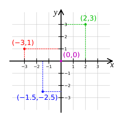
Cartesian coordinate system
K. Bolino, public domain, via Wikimedia Commons
fx, fy, fxy
As explained in fragments, Punctual expressions are evaluated for each fragment. For a given fragment, fx is the x-coordinate of that fragment, fy is the y-coordinate, and fxy is a list with both coordinates.
The next examples are some creative ideas one can explore using only coordinates and basic mathematical functions.
Dividing the screen in 10 vertical gradients:
5 * (fx % 0.2) >> add;
The modulus fx % 0.2 (see mathematical functions for more information) makes 10 stripes from 0 to 0.2 (10 as fx goes from -1 to 1). Then, we multiply by 5 to rescale the value to a 0 to 1 range.
Color patterns
Here we are using three simple formulas to get each of the three RGB channels directly from the coordinates of each fragment.
-- Try changing abs by unipolar
abs [fx, (-1)*fy, (fx+fy)/2] >> add;
unipolar $ (-1)*fx++fxy >> add;
[unipolar $ sin fx, 1 - abs fy, unipolar $ cos fx] >> add;
There are a lot of formulas that allow you to make cool gradients as a starting point for more complex transformations.
See Colors for some ideas on using other colors spaces aside from RGB.
Using punctual to draw mathematical functions:
A typical mathematical function has the form y=f(x), where f(x) is a formula that specifies how to get the y coordinate from the x coordinate. So, for any x, we draw a point at coordinates (x, f(x)).
Using this method we can draw a lot of mathematical functions (here, the zoom is only used to see a bit more of the resulting graph):
zoom 0.4 $ point [fx, cos fx] >> add;
zoom 0.4 $ point [fx, log $ abs fx] >> add;
zoom 0.4 $ point [fx, fx*fx] >> add;
Another way to do the same is by using the between function (see Mathematical functions).
In essence, between receives two values and a graph and returns 1 if the graph is between the two values, or else 0.
Remember that this is evaluated independently for each fragment, so in the next example, for any fragment (fx,fy) we’ll draw white if and only if fy is almost equal to cos fx. The 2*px is the margin that fy can be away from cos y and still be white, and determines the wideness of the line we’ll draw. As explained a bit later, px is the fragment’s height:
zoom 0.4 $ between [cos fx-2*py, cos fx+2*py] $ fy >> add;
We can use evolve these ideas to create interesting patterns:
point [fx, osc 0.09*cos (fx*fy*15*(2+osc 0.32))] >> add;
0.98 * fb >> add;
px, py, pxy
Depending on the screen resolution and the window’s size, pixels on Punctual will have a specific dimensions expressed in the Punctual coordinate system.
You can access a pixel’s width with px and a pixel’s height with py. pxy is a shortcut for [px, py]. This is usually used to draw thin lines, as in the following example, or the ones on the previous section:
zoom 0.4 $ circle [fx, fx*fx] $ 4*px >> add;
aspect, fit
aspect is the ratio between the width and height of the window, so, if you don’t change the window size (or use fit), it’s a constant.
To “see” its value, we can try something like this:
[0.3*aspect,0,0] >> add;
Now, change the window size, and you should see how the background is redder as the width height ratio increases, and darker as it decreases.
fit can be used to rescale the x coordinates in order to change the aspect ratio of the result. When doing this, the visible coordinates on the x-axis no longer will be on the range -1 to 1 (unless fit aspect is specified, which is the same as doing nothing).
The most obvious way of using fit is to correct the aspect of geometric shapes, so a circle draws like a circle, and so on:
fit 1 $ circle 0 0.3 >> add;
fit 1 $ rect 0 0.5 >> add;
Another useful application of fit is to scale an external source (an image, a video, or the camera output) to fit the screen, or a particular portion of the screen:
fit (0.5*aspect) $ move [1, 0] $ img "https://upload.wikimedia.org/wikipedia/commons/d/d4/Karl_Marx_001.jpg" >> add;
fit (0.5*aspect) $ move [-1,0] $ img "https://upload.wikimedia.org/wikipedia/commons/2/21/Friedrich_Engels_portrait_%28cropped%29.jpg" >> add;
In this example, we took images of the Communist Manifesto authors from Wikicommons, and made each one of them to occupy the half of the window, independently from its size.
Same idea, but we divide the window in two horizontally:
fit (2*aspect) $ move [0,-1] $ img "https://upload.wikimedia.org/wikipedia/commons/8/87/Tundra_in_Siberia.jpg" >> add;
fit (2*aspect) $ move [0,1] $ img "https://upload.wikimedia.org/wikipedia/commons/2/2d/Picea_glauca_taiga.jpg" >> add;
Can we combine both previous examples to divide the window in four equal-sized parts? The answer is yes, as aspect is modified just when fit is executed:
fit (0.5*aspect) $ fit (2*aspect) $ move [-1,1] $ img "https://upload.wikimedia.org/wikipedia/commons/2/2d/Picea_glauca_taiga.jpg" >> add;
Now, these last examples show the most standard uses of fit, but you can also use it in many creative ways.
For example, we can apply an oscillator to the aspect ratio to deform the image periodically:
fit (osc 0.2) $ circle 0 0.8 >> add;
Now, evolving this example, we can create beautiful patterns:
spin [saw 0.2, (-1)*saw 0.2] $ fit (8*osc (0.5*cps)) $ tilexy [4,seq [1,4,8,16]] $ circle 0 0.8 * [0.8,0,0.8]>> add;
0.8 * fb >> add;
Here, we are synchronizing the fit oscillator to the beat, and increasing its range to -8 to 8. We are also drawing a lot more circles using tilexy. The replication over the y-axis changes over time, due to the use of seq. Finally, the spin with to graphs as first argument, duplicates the whole set and made each of the copies rotate in opposite directions.
Polar coordinates
In the polar coordinate system, each point in the plane also has two coordinates, but they are the distance to the pole (the center of the window, analogous to the origin in Cartesian coordinates), and the angle from the horizontal ray that goes from the pole to the right (called polar axis), measured in radians.
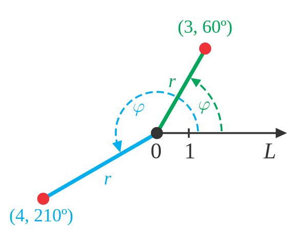
Polar coordinate system
Monsterman222, CC BY-SA 3.0, via Wikimedia Commons
fr, ft, frt
In the same way that fx, fy and fxy allow to get fragment coordinates in the Cartesian system, fr, ft and frt are the fragment coordinates in the polar system.
fr is the distance from the pole, and is equivalent to dist 0 or dist [0,0].
Note that if we only move through one of the axis, fr goes from 0 to 1, but can be larger. The point at [1,1] has a fr of approximately 1.41, that is the square root of 2 (by the Pythagorean theorem).
ft is the angle from the reference ray, which is the right part of the horizontal axis. In Punctual, this angle goes from -π to π radians. This is important, as many times you’d like to rescale this range to a [-1,1] range or [0,1] range, in order to use it in other parts of your code:
- To a [-1,1] range:
ft/pi. - To a [0,1] range:
linlin [(-1)*pi, pi] [0,1] ftorunipolar $ ft/pi.
Next examples are similar to the ones of the Cartesian coordinates section, but the result can be quite different when using polar coordinates.
20 radial gradients:
fit 1 $ 10/pi*(ft % (pi*0.1)) >> add;
Or concentric gradients:
fit 1 $ 10 * (fr % 0.1) >> add;
Color patterns:
r << fr/1.4;
t << ft/pi;
[1-r, abs t, abs $ r/ft] >> add;
r << fr/1.4;
t << ft/pi;
[1-r, abs t, abs $ fx*fy] >> add;
Note how fr and ft are rescaled to keep the red and green coordinates from 0 to 1.
Mathematical functions:
Not so obvious as with Cartesian coordinates, but it’s possible to build interesting shapes using the same ideas:
fit 1 $ point [fx, sin ft] >> add;
For each fragment, draw only the points where y matches the sine of the angle. This results in a circumference of radius 1 (by definition of the sine function, the sine of an angle is the y coordinate of the corresponding point on the circumference of radius 1), and a line at x=0, as the sine of 0 (or π) is 0.
The missing central part of the line is due to rounding errors. Actually, point is a small circle, so it’s visible if some fragment is near enough the specified coordinates. That explain why the circumference has some wideness. Now, as we get closer to the origin, a little change in coordinates radically changes the angle, and that’s why there isn’t any point there which sine is near enough to the y coordinate.
Similarly: fit 1 $ between [sin ft - py, sin ft + py] $ fy >> add;.
dist, prox
dist is the distance of a fragment to a given position.
prox is the opposite of dist, the idea of proximity of a fragment to a given position. prox is calculate such as two opposite screen points have a proximity of 0, and one point has a proximity of 1 to itself.
Let’s take for example [1,1] and [-1,-1] as two point that are as far away from each other as it is possible in the initial visible screen. The distance between them, per the Pythagorean theorem, is the square root of 8, that is approximately 2.828427. prox is computed as (2.828427-dist[x,y])/2.828427, clamped to be between 0 and 1.
One very usual way of using prox is to create masks. Visuals can get quite bright easily, and this can make it difficult for you or the people you are jamming with to see the code on the screen.
You can create a mask in order to keep the borders of the screen relatively clear and focus the visuals on the center:
a << 1;
m << prox 0 ** 4;
a*:m >> add;
Here, a is the annoying graph, in this case a completely white screen. m is the mask, calculated as the proximity to the origin, and raised to the power of 4.
Note that, as all proximities lies between 0 and 1, as we increase the power, the resulting numbers will be nearer to 0.
Finally, we multiply a and m, point to point, deeming each fragment according to the proximity it has to the center.
Following there are some examples on how can we use dist and prox in different creative ways:
- Color patterns depending on the distance of each fragment to certain coordinates:
[dist [0.5,0], prox [-0.6,-0.3], dist [-0.3,0.3]] >> add;
- Deform an image:
i1 << img "https://upload.wikimedia.org/wikipedia/commons/0/0c/Golden-eyed_tree_frog_%28Agalychnis_annae%29_1.jpg";
tilexy [prox [0.5,0], 3*dist [0,0.2]] $ i1 >> add;
Here we use tilexy (see geometric transformations) to deform the image, as the value of tile is different for each fragment.
We can add some audioreactiveness (see audio reactive visuals) to the last pattern to make it a bit more interesting:
i1 << img "https://upload.wikimedia.org/wikipedia/commons/0/0c/Golden-eyed_tree_frog_%28Agalychnis_annae%29_1.jpg";
tilexy [prox [ihi,0], 3*dist [0,ilo]] $ i1 >> add;
From Cartesian to polar and viceversa
There are a bunch of functions that are meant to transform coordinates from the Cartesian system to the polar system or viceversa:
xyrt: from Cartesian to polar.
To understand this function let’s look at the following example:
c << [1,osc 0.1];
fit 1 $ [circle c 0.1, circle (xyrt c) 0.1] >> add;
The red circle stays at x=1 and moves vertically, from y=-1 to y=1 due to the oscillator.
The cyan circle is very similar, but we’ve applied xyrt to its center coordinates. That means that these coordinates are transformed to polar coordinates. So, looking at the first circle and thinking in how this movement affects the angle and radius from the center, we see that the angle moves from -pi/4 to pi/4, that is from approximately -0.79 to 0.79. The radius moves from the square root of two (1.41) at the top, then decreases until it get to 1, just on the horizontal axis, and then increases again to 1.41 at the bottom.
Now we take these two coordinates, but read them as Cartesian coordinates (note that xyrt calculates the polar coordinates, but doesn’t apply any real geometric transformation like setfxy does). So, the result is a circle which x coordinate moves from 1.41 to 1 then again to 1.41, and which y coordinate moves from -0.79 to 0.79.
Let’s add a few reference lines to check our calculations:
c << [1,osc 0.1];
fit 1 $ [circle c 0.1, circle (xyrt c) 0.1] >> add;
mono $ fit 1 $ hline [-0.79, 0.79] px >> add;
mono $ fit 1 $ vline [1,1.41] px >> add;
As a side note, see how the first example can be rewritten shorter using the ++ operator from the combining graphs section:
c << [1,osc 0.1];
fit 1 $ circle (c++xyrt c) 0.1 >> add;
xyr, xyt
These two functions are nearly identical to xyrt, but they only return one of the two coordinates, the radius or the angle respectively.
Following the previous example:
c << [1,osc 0.1];
fit 1 $ [circle c 0.1, circle [xyr c,0] 0.1] >> add;
mono $ fit 1 $ vline [1,1.41] px >> add;
c << [1,osc 0.1];
fit 1 $ [circle c 0.1, circle [0,xyt c] 0.1] >> add;
mono $ fit 1 $ hline [-0.79, 0.79] px >> add;
rtxy: from polar to Cartesian.
This is the opposite from xyrt: it takes coordinates in the polar system and returns the equivalent in the Cartesian system.
c << [1,pi*osc 0.1];
fit 1 $ zoom 0.25 $ circle (c++rtxy c) 0.1 >> add;
The red circle keeps its x coordinate at 1 and oscillates between -π and π on the y coordinate (note the zoom in order to see all its movement).
The cyan circle takes the 1 as its distance from the origin, and changes the angle, so it keeps moving around the origin, always at the same distance.
I find that rtxy is the most usable of the whole family to create cool visual effects.
In the next example, let’s start with this:
l << [2 .. 20]/10;
c << [l*:osc 0.12*osc 0.13, pi*osc 0.1*osc 0.11];
zoom 0.25 $ circle c 0.1 >> add;
These are a bunch of circles that move together in a somewhat irregular way due to the multiplications of oscillators at different frequencies.
The first bit ([2 .. 20]/10) uses a list expansion to create the x coordinate for each circle, from 0.2 to 2, going in steps of 0.1.
The y coordinate is common to all circles, and oscillates from -π to π.
Next step is just take all the circle’s center coordinates and read them as polar coordinates.
l << [2 .. 20]/10;
c << [l*:osc 0.12*osc 0.13, pi*osc 0.1*osc 0.11];
circle (rtxy c) 0.1 >> add;
Now, we apply some basic geometric transformations, using combinations of fx, fy, ft and fr to twist the circles geometry:
l << [2 .. 20]/10;
c << [l*:osc 0.12*osc 0.13, pi*osc 0.1*osc 0.11];
fit 1 $ spin (fr*4) $ move [ft*fx*0.3,ft*0.1] $ circle (rtxy c) 0.1 >> add;
Finally, let’s add some repetition in the middle to create more elements:
l << [2 .. 20]/10;
c << [l*:osc 0.12*osc 0.13, pi*osc 0.1*osc 0.11];
fit 1 $ spin (fr*4) $ tile 4 $ move [ft*fx*0.3,ft*0.1] $ circle (rtxy c) 0.1 >> add;
Playing with circles and polar coordinates is fun! In the last example, all the circles were moving like a whole. Can we make each one to move separately from the others?
Let’s start with our circles forming a bigger circumference around the center:
t << linlin [0,1] [0, 2*pi] $ [0 .. 50]/50;
fit 1 $ circle (rtxy [0.5, t]) 0.1 >> add;
Here we use a list expansion for the circles angles, just like in the last example, and rescale it from a 0 to 1 range to a 0 to 2π using linlin, just because it’s easier to think from 0 to 1.
Then draw all the circles using polar coordinates, at a fixed distance from the origin of 0.5.
Let’s made the circles spin:
t << linlin [0,1] [0, 2*pi] $ [0 .. 50]/50;
o << pi * saw 0.1;
fit 1 $ circle (rtxy [0.5, t+:o]) 0.1 >> add;
Here, o is an oscillator that goes from -π to π, and when it reaches π it starts again from -π. We add this oscillator to each angle, and the result is that all the circles spin together.
Finally, let’s apply an oscillator to the radius too, but this time, each circle will have a distinct frequency, so they will move apart from each other. We make this by using t to modify the oscillator frequency in the bit osc (0.1*t).
Now, we have a list of radius and a list of angles, and we need to link them together: the first radius with the first angle, the second radius with the second angle, and so on. This is just what the zip function from combining lists does.
As a final touch, we use mono to combine all channels into one, which make all circles white:
t << linlin [0,1] [0, 2*pi] $ [0 .. 50]/50;
o << pi * saw 0.1;
fit 1 $ mono $ circle (rtxy $ {osc (0.1*t), t+:o}) 0.1 >> add;
rtx, rty
These two functions are nearly identical to rtxy, but they only return one of the two coordinates, the x or y coordinate respectively.
r << unipolar $ osc 0.03;
t << pi*osc 0.07;
fit 1 $ circle [r,t] 0.1 >> add;
red << circle (rtxy [r,t]) 0.1;
green << circle {rtx [r,t], 0} 0.1;
blue << circle {0, rty {r,t}} 0.1;
fit 1 [red,green,blue] >> add;
In this example, r oscillates from 0 to 1, and t from -π to π. There are a total of four circles:
- White:
randtare interpreted as Cartesian coordinates x and y. - Red:
randtare read as polar coordinates. - Green:
randtare polar coordinates, but only used to calculate the resulting x position. - Blue: same as green, but only the y position is calculated.
Examples
10 ways of drawing a circumference of radius 1
Just to see the flexibility of Punctual and different ways to use coordinates, let’s think of different ways to draw a circumference of radius 1.
Probably the easiest way: let’s paint white (1) all fragments whose radius is 1, pixel more, pixel less:
between [1-px, 1+px] fr >> add;
As the radius is no more than the distance to the origin, this is equivalent:
between [1-px, 1+px] $ dist 0 >> add;
Also, it’s possible to make this calculation explicit, using the Pythagorean theorem:
between [1-px, 1+px] $ sqrt $ fx*fx+fy*fy >> add;
Next is a similar approach, but without using between. Here, on one hand we take all fragments whose radius is a bit lesser than one, and on the other the fragments whose radius is a bit greater than one. What we want is the intersection of those two, so we multiply the graphs (the result will be one only if both graphs have a one on that fragment).
(fr <= 1+px) * (fr >= 1-px) >> add;
Another way of thinking this is by using the mathematical function of a circumference. For any x, we have to paint only the y that follow the formula x^2 + y^2 = 1. Isolating the y we get:
f << [-1,1]*(sqrt $ 1-fx*fx);
mono $ point [fx, f] >> add;
Note how the square root is multiplied by [-1,1] in order to take both roots.
Now we can take both ways of thinking and mix them. We’ll paint white only those fragments whose x-coordinate is near the computed y for the circle at that x:
c << sqrt (1-fy*fy);
between [c-px, c+px] $ abs fx >> add;
In the last example, we are only taking the positive root of the square root, but are taking the absolute value of x to make the graphic symmetrical.
Yet another way of thinking this problem: we already have a function that draws circles. Let’s tweak it to draw a circumference instead.
In this example, we draw a circle of radius 1, and then take off a slightly smaller circle:
(circle 0 2) - (circle 0 $ 2-2*px) >> add;
Next is mathematically equivalent to the last one, but we get here with another way of thinking. We can draw the inner part of the circumference with a circle, and also the outer part with an inverted slightly bigger circle (using 1- to invert the result, as it is all 0 and 1). So, we have obtained just the invert of what we want, so we invert the result again:
1-(1-circle 0 (2+2*px) + circle 0 (2-2*px)) >> add;
Finally, a last way to solve the problem is by transforming coordinates from Cartesian to polar. If you think about it, a circumference has a very easy representation on polar coordinates, as one of them (the radius) is constant.
This is exactly what vertical and horizontal lines are: a graph where one of the two coordinates is constant.
So we can draw a vertical line, and then think of it a circumference in polar coordinates, so when we interpret the x as the radius and the y as the angle, we get a circumference:
setfxy frt $ vline 1 px >> add;
Similarly, we can use a horizontal line, and the we need to interpret the x coordinate as the angle, and the y coordinate as the radius:
setfxy [ft,fr] $ hline 1 px >> add;
Bonus track: set feedback to 100% and use a point like it is a pencil:
spin (saw 0.06) $ point [0,1] >> add;
fb >> add;
Implementing Hydra functions
As explained in the Overview, Hydra is a popular language for live-coding visuals. One key difference between Hydra and Punctual is that Punctual operates at a slightly lower level than Hydra.
This means that while it is possible (though not always straightforward) to reimplement many Hydra functions using Punctual, the reverse is not necessarily true.
Let’s develop a couple of examples to illustrate this.
- Implementing Hydra’s
osc()function:
Hydra’s osc() function draws a sine wave, visualized from above. When the sine wave is far away (low), the visualization appears black, and as it gets closer, it turns white.
In Punctual, this can be expressed using unipolar $ sin (fx*freq), where freq determines the number of sine wave repetitions. To fully mimic Hydra’s osc(), we need to adjust the coordinates and use unipolar fx instead of fx: unipolar $ sin (unipolar fx*freq).
Hydra’s osc() also moves horizontally over time. We can achieve this by adjusting the phase of the sine wave based on the elapsed time:
unipolar $ sin ((unipolar fx+sync*time)*freq);
Hydra uses 60 as the default frequency and 0.1 for the sync parameter. Applying these values, the Punctual expression becomes:
unipolar $ sin ((unipolar fx+0.1*time)*60) >> add;
This expression recreates the behavior of Hydra’s osc() function in Punctual.
- Implementing
osc().kaleid():
Now that we have our version of Hydra’s osc() function, we can extend it with some transformations, such as kaleid().
In this example, we are reimplementing the Hydra expression osc().kaleid(5).out().
The core idea of kaleid(5) is to apply a geometric transformation (using setfxy) by which we take an arc of a fifth of the whole circle and copy it five times, filling the entire screen. Additionally, we need to rotate our arc so that the different parts align correctly, and apply a translation because Hydra’s kaleid() copies the upper left part of the image but draws it at the center.
This is a possible implementation:
hosc << unipolar $ sin ((unipolar fx+0.1*time)*60);
k << ft % (2*pi/5);
setfxy (rtxy [fr, k]) $ spin ((-1)/5) $ move 0.5 hosc >> add;
- First line: This is our version of Hydra’s oscillator,
osc(), which creates a sine wave pattern that moves horizontally over time. - Second line: Here,
kis defined. It represents the new angle for each fragment, and the modulus (%) operator is used to map any fragment to the first fifth of the circle. This is the key to the whole kaleidoscope effect. - Third line: This line combines several transformations:
move 0.5 hosc: Moves the oscillator 0.5 units in each coordinate, effectively shifting the top-left corner of the screen to the center.spin ((-1)/5): Rotates one-fifth of the whole circle, ensuring that each part of the pattern matches up seamlessly.setfxy (rtxy [fr, k]): Applies the geometric transformation. Note thatsetfxy (rtxy frt) somethingis an identity transformation, as it retains the radius and the angle. In our case,kis assigned as the new angle, effectively creating the kaleidoscope effect by repeating and rotating the pattern.
This implementation effectively mimics Hydra’s osc().kaleid(5).out() by using Punctual’s lower-level functions to achieve the same visual result.
setfxy is so flexible that we could include the move, spin and rtxy operations inside the setfxy transformation making the whole transformation in only one step:
hosc << unipolar $ sin ((unipolar fx+0.1*time)*60);
k << ft % (2*pi/5)-pi/5;
setfxy (fr*[cos k, sin k]-0.5) hosc >> add;
Of course, this is complicated to deduce, but as Hydra is free software, we can look up the original kaleid implementation and translate the code to Punctual.
7 - Colors
Color in Punctual is intimately related to channels.
Colors and output notations
Depending on the output notation used, channels are interpreted as colors in different ways (see output notations):
add,rgb,mul: first channel is red, second green, and third blue. If there is less than 3 channels, they are read following these rules:- One channel: the same value is used for the three base colors, resulting in a gray level, from 0 black to 1 white.
- Two channels: the first channel is red, the second is used for both blue and green, resulting in cyan.
- More than three channels: every 3 channels are a group of red, green, blue, any excess is read as in the previous rules. So, for example, a 5-channel signal would be red-green-blue-red-cyan, and a 4-channel signal red-green-blue-white.
blend,rgba: first channel is red, second green, third blue, and forth is alpha (transparency). Chanel matching works in the same way asadd, but with four output channels, and can be confusing. For example,circle [0,0,0.1,0.1] 0.1 >> blend;is a 2-channel signal. The first circle is red, but it will have 0 on the alpha channel, so it’s invisible. The second circle is cyan and visible, asg,bandaare joined. Therefore, usingblendwith an arbitrary number of channels won’t produce many interesting results.
Basic usage
Most of the times, we’ll create a 1-channel signal and then convert it into a 3-channel signal to get color in the RGB color space. To do this, we only need to multiply our signal by a three elements list. Due to Punctual’s combinatorial nature, our signal will be split in three channels, being the same on all of them, except for the multiplying factor on each one:
circle 0 0.2 * [0.8,0,0.8] >> add;
Note that each color component receives a value from 0 to 1. There is no problem in sending lower or higher values, but they will always be trimmed to this range.
The following table shows the codes corresponding to some basic colors in both the RGB and HSV color-spaces:
| Name | RGB | HSV |
|---|---|---|
| Black | 0,0,0 | 0,0,0 |
| White | 1,1,1 | 0,0,1 |
| Red | 1,0,0 | 0,1,1 |
| Lime | 0,1,0 | 0.33,1,1 |
| Blue | 0,0,1 | 0.67,1,1 |
| Yellow | 1,1,0 | 0.17,1,1 |
| Cyan | 0,1,1 | 0.5,1,1 |
| Magenta | 1,0,1 | 0.83,1,1 |
| Silver | 0.75,0.75,0.75 | 0,0,0.75 |
| Gray | 0.5,0.5,0.5 | 0,0,0.5 |
| Maroon | 0.5,0,0 | 0,1,0.5 |
| Olive | 0.5,0.5,0 | 0.17,1,0.5 |
| Green | 0,0.5,0 | 0.33,1,0.5 |
| Purple | 0.5,0,0.5 | 0.83,1,0.5 |
| Teal | 0,0.5,0.5 | 0.5,1,0.5 |
| Navy | 0,0,0.5 | 0.67,1,0.5 |
| Orange | 1,0.65,0 | 0.11,1,1 |
| Turquoise | 0.25,0.88,0.82 | 0.48,0.71,0.88 |
| Violet | 0.93,0.51,0.93 | 0.83,0.45,0.93 |
| Pink | 1,0.75,0.8 | 0.97,0.25,1 |
| Lavender | 0.9,0.9,0.98 | 0.67,0.08,0.98 |
Of course, things get interesting when we use non constant expressions for the color channels.
Color changes by space
Creating color patterns involves playing with coordinates (fx, fy, fr, ft) and mathematical operations (abs, unipolar, %, and trigonometric functions are pretty useful for this).
There are plenty examples of this on the sections dedicated to Cartesian coordinates and polar coordinates.
color << [abs fx, unipolar fy, fr]/8;
(mono $ fit 1 $ spin (saw [0.03, -0.03]) $ tilex 15 $ vline 0 0.06) * color >> add;
0.95 * fb >> add;
- Red component is defined as
abs fx, so it’s higher on the right and left sides. - Green component is defined as
unipolar fy, so it’s 0 at bottom and 1 at the top of the window. - Blue component is
frso it get higher as we got far from the center. - Note the use of
mono. The signal (before color is applied) it’s a 2-channel signal, due to the list inspin, so when multiplied by the 3-channel color, it would result in a 6-channel signal. The use ofmonoconverts the 2-channel signal into a 1-channel, so it get lighter on the CPU, even though the visual result is the same. - Also note the use of parenthesis to make sure color is applied after the rest of the expression is evaluated. Otherwise, it will only affect the
vlinebit. Withmonothis would result in only white lines (as the 3-channel color would be squashed into a 1-channel signal). Withoutmono, the pattern is completely different, as the color is first applied to the vertical line, and then the other transformations take place.
Color changes by time
There are several ways to make a color pattern evolve through time. One of the easiest is using oscillators (osc, tri or saw), but remember that by default oscillators go from -1 to 1, and a color component from 0 to 1, so many times you will be using unipolar or abs to rescale the values. The ~~ operator is also useful when you don’t want a component to reach all values from 0 to 1 (for example, 0.5 ~~ 0.8 $ osc 0.1 will oscillate only between 0.5 and 0.8).
When using oscillators, you can use a frequency that depends on cps to synchronize the oscillator to the beat (see audio-reactive visuals).
[unipolar $ osc (cps/2), 0.5*abs (tri (cps/4)), 0.3 ~~ 1 $ saw (cps/6)] >> add;
saw is useful to make a flash at each beat. Supposing a 4/4 beat, unipolar $ saw (cps*4) will start at 0 at the beat’s start and end at 1 just when the next beat hits. You can use 1 - unipolar $ saw (cps*4) or the equivalent expression 1-4*(beat%0.25) to make the flash start at 1 with the beat and then fade out. The example is slowed down to reduce the flickering:
slow 4 $ [1-beat%1, 1-4*(beat%0.25), 0] >> add;
You can use late and early to change the phase of an oscillator (see Time shifting functions):
[osc cps, 0, late (cps/2) $ osc cps] >> add;
Note that we haven’t used unipolar here, so really both oscillators are going all the way to -1. We can take advantage of this:
fit 1 $ (1-fr)*:[osc cps, 0, late (cps/2) $ osc cps] >> add;
Color mixing
Any light based device uses an additive color mixing. When two lights are mixed, the frequencies of both are visible, resulting in a clearer color. If enough frequencies are added, the result is white.
In contrast, when using pigments, color mixing is subtractive. Each pigment captures certain light frequencies and reflects the rest. As we add more pigments, more frequencies are captures, and the color is darker, leading to black if we mixed enough pigments.
So by default, Punctual uses an additive color mixing:
iline [-1,1,-1,0,-1,-1] [0,0] 0.2 >> add;
This graph has 3 channels, so the first line is red, the second line is green, and the third one is blue.
Note how colors are mixed together when the lines intersect. For example, when the red and green line intersect the resulting color is yellow ((1,0,0)+(0,1,0)=(1,1,0)). At the center, where the three lines come together, the resulting color is white ((1,0,0)+(0,1,0)+(0,0,1)=(1,1,1)).
An additive color mixing system is prone to end up with a white screen when there are many elements interacting, especially when using feedback.
There are a few tricks we can use to avoid this and still be able to have a lot of different elements interacting.
- Using subtractive color mixing.
Although our computer uses light to show us information and so it’s a naturally additive device, we can simulate a subtractive system by using some calculations.
First of all, let’s say that talking here about subtractive color models is a language abuse. This is a very complex problem that involves the chemical and physical properties of pigments and materials, and are impossible to recreate in a live-coding context.
Fortunately, we don’t need realism. We are just looking for some simple enough calculation we can apply when mixing color that make sure the result won’t be white when things get messy.
Also, we can’t change how colors are automatically mixed when using patterns like the three lines example above. But we can control how colors are mixed when creating patterns, and this by itself it’s quite useful.
Let’s take a very simple approach and say that we mix two colors, c1=(r1,g1,b1), c2=(r2,g2,b2), in a subtractive way by this formula:
c3=(1-abs(r1-r2), 1-abs(g1-g2), 1-abs(b1-b2))
This simple formula works well for basic colors: magenta and yellow will result in red, magenta and cyan will give blue and so on.
In Punctual, we can write the above formula by the very simple expression:
c3 << 1 - (abs $ c1-:c2)
Note how the -: operator takes care of all components at once. Also, avoid using -, because due to the combinatorial nature of this operator you will end up with, you guessed it, white.
Now we can play with complex color patterns and never end up with a white screen:
c1 << unipolar $ osc [0.07, 0.11, 0.06];
c2 << unipolar $ osc [0.05, 0.09, 0.1];
1-:(abs $ c1 -: c2) >> add;
This is just an example formula, we can take other simple ideas (absolutely non-realistic, but our aim is another one): abs $ c1 -: c2, c1*:c2 and so on…
Let’s create a more extreme example. In this case, abs $ c1 -: c2 is used, as it renders darker colors:
a << spin (saw 0.02) $ tilexy [8,4] $ unipolar (spin (saw 0.13) fx);
b << spin ((-1)*saw 0.03) $ tilexy [16,8] $ unipolar $ (spin (saw 0.15) $  fx*fy);
c1 << a*:[unipolar $ osc 0.1,0,unipolar $ osc 0.15];
c2 << b*:[unipolar $ osc 0.3,unipolar $ osc 0.5,0];
c3 << abs $ c2 -: c1;
abs $ c3 -: (spin (saw 0.05) $ zoom 2 fb) >> add;
There a lot of code here, but note that basically, a and b are two patterns of numbers (only one channel per fragment) that depend on fx and fy and spin as time passes.
c1 and c2 are the product of a and b with an oscillating color. If we visualize c1 or c2 by themselves, the pattern is quite simple.
Now, c3 is the mixing of c1 and c2. If we display c3, the mixing of the other two patterns is obvious, but we can clearly see the different colors, as the screen never collapses to white.
Finally, we use feedback to take the last frame, apply some transformations to it, and remix it with c3. The resulting pattern is quite complex, but again, it never gets too bright.
- Using transparency.
One simple way to keep things under control, especially when using high amounts of feedback, is to apply some transparency to your patterns.
Note the difference between these two examples:
0.99 * fb >> add;
co << [abs fx, unipolar fy, fr];
s << slow 10 $ seq [0,0.2,0.4,0.7];
z << (xyrt $ (2+fr)*(abs $ 1-fx)*fy);
sp << [osc 0.035*saw 0.3, (-1)*osc 0.026*saw 0.03];
(mono $ fit 1 $ spin s $ zoomxy z $ spin sp $ tilex 15 $ vline (fy*0.5) 0.06) * co >> add;
0.99 * fb >> add;
co << [abs fx, unipolar fy, fr, 0.8];
s << slow 10 $ seq [0,0.2,0.4,0.7];
z << (xyrt $ (2+fr)*(abs $ 1-fx)*fy);
sp << [osc 0.035*saw 0.3, (-1)*osc 0.026*saw 0.03];
(mono $ fit 1 $ spin s $ zoomxy z $ spin sp $ tilex 15 $ vline (fy*0.5) 0.06) * co >> blend;
Both are the same being the only difference that in the second one we set a 0.5 value to the alpha channel.
In the first example, the screen gets practically white, with some cyan and magenta artifacts forming a vertical and an horizontal line respectively.
In the second example, we can clearly see the patterns that the moving lines are creating, and the screen never gets too bright, even with the high amount of feedback applied.
Note that the order of the operations is important. We need to use blend after add, as seen in Output Notations.
- Gradients.
c1 << [1,0,0];
c2 << [1,0,1];
x << unipolar fx;
c2*x +: c1*(1-x) >> add;
Color spaces
You can use two color spaces in Puntual: RGB and HSV. So far, we’ve been using the RGB color space.
HSV color space is best understood as a mixing of paints. Informally, the hue value represents which color we choose, saturation is the amount of pigment of the chosen color we add, and value is the amount of white light we project on our object.
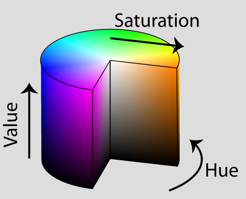
HSV Color space
Jacob Rus, CC BY-SA 3.0, via Wikimedia Commons (edited)
So, for example, if we fix 0.8 (purple) as the hue, and 0.5 as the value, with 0 saturation we get a medium gray and, as we add more and more saturation, the amount of purple increases. Now, if we start to change the value, we can pass from a completely black color with 0, to a very bright purple when we get to 1.
Punctual has functions to isolate one of the channels, translate from one color space to the other, and the combination of these two operations.
rgbr, rgbg, rgbb
rgbr,rgbg,rgbb: use these functions to isolate one of the three channels in an RGB expression. If the input signal has more channels, the result is one channel out of three.
In the next example, we take the red channel of a first video, and the green channel of a second one, then we combine them:
v1 << rgbr $ vid "https://upload.wikimedia.org/wikipedia/commons/4/4f/Midway_Atoll_-_Bird_Sightings_-_Mar-Apr_2015.webm";
v2 << rgbg $ vid "https://upload.wikimedia.org/wikipedia/commons/2/21/Sparrow_hawk.webm";

[v1,v2,0] >> add;
The next example is based on a previous example about subtractive colors, adding only a move call. Each fragment is moved through the x axis according to its red component. This breaks the regularity of the previous example, creating more interesting and variable patterns:
a << spin (saw 0.02) $ tilexy [8,4] $ unipolar (spin (saw 0.13) fx);
b << spin ((-1)*saw 0.03) $ tilexy [16,8] $ unipolar $ (spin (saw 0.15) $  fx*fy);
c1 << a*:[unipolar $ osc 0.1,0,unipolar $ osc 0.15];
c2 << b*:[unipolar $ osc 0.3,unipolar $ osc 0.5,0];
c3 << abs $ c2 -: c1;
move [rgbr c3,0] $ abs $ c3 -: (spin (saw 0.05) $ zoom 2 fb) >> add;
hsvh, hsvs, hsvv
hsvh,hsvs,hsvv: these are synonyms ofrgbr,rgbgandrgbbrespectively. Note that all these functions do is take the first, second or third channels out of every set of three input channels, so it really doesn’t matter if the original input is an RGB color, a HSV color, or any other thing.
rgbhsv, hsvrgb
rgbhsv,hsvrgb: translate a signal from the RGB color-space to the HSV, or vice-versa.
In the following example, the frequencies captured by the microphone are utilized to modulate the hue of horizontal lines. The setfx function is used to transform the default result of ifft into horizontal and symmetrical lines. These intensities are subsequently used as the hue parameter in the HSV (Hue, Saturation, Value) color space, with the saturation and value held constant. The hsvrgb function converts the resulting color into the RGB color space.
hsvrgb [setfx (bipolar $ abs fy) $ ifft, 1, 0.5] >> add;
The following example begins by creating two circles that traverse the screen in a slightly irregular manner. The x and y variables define the coordinates of one circle, and a spin operation with two channels is applied, resulting in the creation of two circles derived from the initial one.
The color of the two circles is determined using the HSV color system. The hue (h) varies over time from 0.5 to 0.7, and the saturation (s) ranges from 0.2 to 0.9. The value is fixed at 0.8. Once the color is defined, it is translated to the RGB color space using hsvrgb. An alpha channel of 1 is then added, as discussed in Using transparency with feedback, to prevent saturation to white when employing extensive feedback.
Next, feedback is introduced into the scene, with its color slightly rotated each frame. This is achieved by translating the feedback from RGB to HSV color spaces using rgbhsv. A small amount is added to the hue, and the resulting color is translated back to RGB before being displayed on the screen. Note that this doesn’t affect the background color, as we are only changing the hue of the feedback. Also, note that we used add before blend, as explained in Output Notations.
x << osc 0.091*osc 0.085;
y << osc 0.07*osc 0.06;
sp << saw [0.013,-0.027];
c << fit 1 $ mono $ spin sp $ circle [x, y] 0.2;
h << 0.5~~0.7 $ osc 0.13;
s << 0.2~~0.9 $ osc 0.003;
co << (hsvrgb [h, s, 0.8])++1;
fc << [0.003,0,0];
hsvrgb $ rgbhsv fb+:fc >> add;
c * co >> blend;
In this final example, an audio-responsive chain of lines is created. The x-coordinates of all segments, denoted by xs, are evenly spaced along the x-axis. The use of [0..32]/32 efficiently generates a sequence of fractional numbers from 0 to 1 in steps of 1/32, and the application of bipolar spreads these numbers across the entire x-axis. The y-coordinates, defined by ys, are determined by taking 33 sample frequencies from the input audio signal. Consequently, the intersection points between the lines move up and down based on their associated frequencies.
The segments are constructed using the chain function and are mirrored across the y-axis by employing setfy [fy, (-1)*fy]. Subsequently, the entire set is slowly rotated.
Color is once again specified in the HSV color space, with a hue oscillating across all possible values, while the saturation and value remain fixed. Similar to the previous example, the color is translated to RGB using hsvrgb, and an alpha channel is added.
The pattern is finalized by introducing feedback and rapidly zooming it in.
l << [0..32];
xs << bipolar $ l/32;
freqs << bipolar $ l/50;
ys << 1.5*(setfx freqs ifft);
ch << spin (saw 0.02) $ setfy [fy, (-1)*fy] $ mono $ chain {xs,ys} 0.02;
co << (hsvrgb [osc 0.3, 0.8, 0.9])++0.7;
zoom 1.02 fb >> add;
ch*co  >> blend;
rgbh, rgbs rgbv, hsvr, hsvg, hsvb
rgbh,rgbs,rgbv,hsvr,hsvg,hsvb: This set of functions is similar torgbhsvandhsvrgb, but each returns only one channel for each set of three.rgbhtranslates from RGB to HSV and returns the hue,rgbsthe saturation, andrgbvthe value. Similarly,hsvr,hsvg, andhsvbtranslate from HSV to RGB and return the red, green, and blue channels, respectively.
This example uses this set of functions to apply a filter to a video. The original video is displayed on the left side of the screen, while color transformations are applied to the right part.
The color transformations occur in the HSV color space. The hue undergoes a slight change by subtracting 0.08 from it. The saturation is significantly increased by multiplying it by 1.8. The value remains unchanged. After applying these transformations, the color is translated back to RGB for display. The result is an otherworldly sensation achieved through simple channel adjustments.
v << vid "https://upload.wikimedia.org/wikipedia/commons/4/4f/Midway_Atoll_-_Bird_Sightings_-_Mar-Apr_2015.webm";
(fx>0) * hsvrgb [rgbh v - 0.08, 1.8*rgbs v, rgbv v] >> add;
(fx<=0) * v >> add;
8 - Oscillators
An oscillator is a device that generates oscillations:
the repetitive or periodic variation, typically in time, of some measure about a central value (often a point of equilibrium) or between two or more different states. — https://en.wikipedia.org/wiki/Oscillation
In Punctual, an oscillator is a function that returns values in the range from -1 to 1, varying through time.
All oscillators take a single argument: the oscillation frequency in hertz (full cycles per second).
osc, tri, saw, sqr
There are four oscillators in Punctual, each with a different pattern:

In the next example, you can see all four oscillators in action. There are four balls, each one moving according to one of the oscillator types along the y axis, and using the same colors as in the previous representation. Each cycle lasts 4 seconds instead of 1:
fit 1 $ (circle [-0.6, osc 0.25] 0.1 * [1,0,0] +:
circle [-0.2, tri 0.25] 0.1 * [0,0,1] +:
circle [0.2, saw 0.25] 0.1 * [1,0,1] +:
circle [0.6, sqr 0.25] 0.1 * [0,1,0]) >> add;
The first circle, in red, uses the osc function and follows a sinusoidal wave. The second one, in blue, uses tri and follows a triangle waveform. The third one, in magenta, uses saw and follows a saw wave, that is, it increases its value from -1 to 1, and then jumps and starts again at -1. The last circle, in green, uses sqr and follows a square wave, taking only the values -1 and 1 for half a cycle each one.
Oscillators are such a fundamental tool in Punctual that you can find examples of them being used across all the sections in this guide.
Summarizing, oscillators can be used to modulate:
- Coordinates
x1 << osc 0.13;
y1 << osc 0.15;
x2 << osc 0.09;
y2 << osc 0.11;
line [x1,y1] [x2,y2] 0.001 >> add;
fit 1 $ circle [x1*x2, y1*y2] 0.2 >> add;
line [tri fx, tri fr] [tri fy, tri fr] 1 >> add;
- Transformations
l << [5 .. -6]/100;
mono $ spin (saw l) $ hline 0 0.001 >> add;
- Colors
fit 1 $ circle 0 1 * (0.5 ~~ 1 $ sqr [0.73, 0.81, 0.65]) >> add;
- Sizes
fit 1 $ circle 0 (2*:(unipolar $ sqr (0.5+fx*fy*5))) >> add;
hline 0 (0.2*(abs $ osc (0.2*abs fx))) >> add;
- Other oscillator frequencies
0.99 * fb >> add;
f<<[0.1,0.11..0.2];
(mono $ circle [osc (0.01*:osc f), osc (0.01*:osc f)] 0.1) * [1.2-fr,0,0.6,0.3] >> blend;
- Between a set of values (see
seqbelow)
Changing the phase of an oscillator
The phase is the position on the cycle of an oscillator where it begins its movement. Two oscillators can have the same frequency and amplitude, but different phase, and then one is displaced respect the other:

At the moment, the easiest way to change the phase of an oscillator is by using early or late:
o << osc 0.1;
(between [-1,0] $ fx) * o >> add;
(between [0,1] $ fx) * (late 5 o) >> add;
Here, the o oscillator has a frequency of 0.1, that is, it completes a cycle every 10 seconds. The second version has the same frequency, but it starts 5 seconds later, so it will be in antiphase with the first one.
The same idea can be applied to the other oscillators.
o << tri 0.1;
(between [-1,0] $ fx) * o >> add;
(between [0,1] $ fx) * (late 5 o) >> add;
o << saw 0.1;
(between [-1,0] $ fx) * o >> add;
(between [0,1] $ fx) * (late 5 o) >> add;
o << sqr 0.1;
(between [-1,0] $ fx) * o >> add;
(between [0,1] $ fx) * (late 5 o) >> add;
seq
seq is a function that acts as a step sequencer. It takes a list of expressions as an argument and iterates through them, choosing one at a time based on the phase of a saw oscillator synchronized to the cycle. This allows for creating rhythmic or patterned variations over time. For example, you can use seq to alternate between different positions, colors, or other properties in a cyclic manner.
s << seq [-0.5,0,0.5];
vline s 0.001 >> add;
Here, the vertical line position changes regularly, taking the values in the list by turns.
Use slow or fast to change the speed of the sequencer, and late or early to change the phase:
s << fast ([1,2]/7) $ seq [-0.5,0,0.5];
spin (late [1,2] s) $ vline s 0.3 >> add;
Next, there is a more complex example. x and y define the center coordinates of a circle. Due to the fast oscillators controlling seq, the circle jumps between four moving points in the screen. r is the circle radius, which changes over time between three values. c is the circle’s color, which is changing over a reduced set of possibilities, due to the three seq functions using different frequency oscillators. Note how the alpha channel is set to 0.7. This, with the feedback set to a full 1, allow the circles in each frame to accumulate on the screen without saturating the color (this technique is explained in the color section), creating the effect that there are four circles moving:
fb >> add;
x << osc 0.17*osc 0.19*(fast 10.2 $ seq [-1,1]);
y << osc 0.16*osc 0.18*(fast 10.6 $ seq [-1,1]);
r << fast 0.34 $ seq [0.1,0.2,0.3];
c << [fast 10 $ seq [0.5,1], fast 108 $ seq [0,0.5,1], fast 114 $ seq [0,0.5,1], 0.7];
fit 1 $ circle [x,y] r * c >> blend;
seq is not limited to single numbers. You can use it to iterate over a list of expressions:
c << fit 1 $ circle 0 0.5;
c2 << slow 4 $ seq [zoom 2 c, move [0.5,0] c];
c2 * [0.3, 0.6, 0.8] >> add;
It is even possible to use multi-channel expressions:
c << fit 1 $ circle 0 0.5 * [0.3, 0.6, 0.8];
c2 << slow 4 $ seq {zoom 2 c, move [0.5,0] c};
c2 >> add;
This last example is equivalent to the previous one, but signals inside seq are multi-channel expressions, as we have applied color to the circle before the seq function. The use of curly braces {} is necessary to correctly mix the signals.
i1 << img "https://upload.wikimedia.org/wikipedia/commons/b/b4/Vaporwave_for_China.jpg";
i2 << img "https://upload.wikimedia.org/wikipedia/commons/4/48/Mao_Tse_tung_in_1965_Color.png";
i3 << img "https://upload.wikimedia.org/wikipedia/commons/b/b6/Mao_Zedong_in_front_of_crowd.jpg";
slow 4 $ fit (seq [1,0.66,0.86]) $ seq {i1,i2,i3} >> add;
spr, sprp
spr (for spread) is similar to seq, but you can define the function that chooses the next value. It takes two arguments: the list of values and the function that will choose the next value. sprp is the pairwise version of spr.
The following code is equivalent to the first example using seq:
s << spr [-0.5,0,0.5] $ saw cps;
vline s 0.001 >> add;
spr and sprp are useful when you want to use another oscillator instead of saw, when you don’t want to align the oscillator to the tempo, or when you want to use a custom function to choose the next value.
Evolving from the last example, we can now start to apply transformations to the feedback. Here, we use spr to apply a spinning effect. But this time, the amount of spinning applied depends on the distance from the center (fr), so fragments on the center rotate to the right, fragments a bit more distant rotate slower to the left, more distance ones to the right again, and the most distant don’t rotate at all:
zoom 1.003 $ spin [spr [0.03,-0.005,0.01,0] $ (bipolar fr)] fb >> add;
x << osc 0.17*osc 0.19*(fast 10.2 $ seq [-1,1]);
y << osc 0.16*osc 0.18*(fast 10.6 $ seq [-1,1]);
r << fast 0.34 $ seq [0.1,0.2,0.3];
c << [fast 10 $ seq [0.5,1], fast 108 $ seq [0,0.5,1], fast 114 $ seq [0,0.5,1], 0.7];
fit 1 $ circle [x,y] r * c >> blend;
9 - Combining graphs
In this section, some of the operators used to combine graphs are studied.
One of the important characteristics of Punctual is its default combinatorial nature. This means that usual arithmetic operators like + or * are combinatorial, and there exists another whole set of operators which are pairwise (+: and *: instead of + and *).
Combinatorial binary operators
A combinatorial operator creates all possibilities that result from combining any channel from the first graph with any channel from the second graph.
For example, [0.1, -0.1] + [0.3, 0.2] results in the expression [0.4, 0.3, 0.2, 0.1], and [0.1, 0.2, 0.3] + [0.3, 0.6] is [0.4, 0.7, 0.5, 0.8, 0.6, 0.9].
The list of combinatorial binary operators is as follows:
- Arithmetic:
+: addition, 8+2=10-: subtraction, 8-2=6*: multiplication, 8*2=16/: safe division. This operator performs division like usual, but if the divisor is 0, the result is defined as 0 to avoid errors. 8/2=4**: exponentiation, 8**2=64.%: modulo. The remainder obtained after dividing the first argument by the second. 8%2=0, 8%3=2.
- Comparison: these operators return 1 if the condition is met and 0 if not.
==: equal to. 8==2=0, 8==8=1/=: not equal to. 8/=2=1, 8/=8=0>: greater than. 8>2=1, 2>8=0, 8>8=0>=: greater than or equal. 8>=2=1, 2>=8=0, 8>=8=1<: less than. 8<2=0, 2<8=1, 8<8=0<=: less than or equal. 8<=2=0, 2<=8=1, 8<=8=1
Let’s start with a very simple example just to see how graphs are combined:
p << [0.1,-0.1]+[0.3,0.2];
--p << [0.4,0.3,0.2,0.1];
circle p 0.1 >> add;
Note that the first and second (commented out) lines are equivalent.
In the next example, a complex pattern of points is created, using list expansions and the combinatorial operators + and *.
The first list has 7 channels, and the second list has 5 channels. This results in p having 35 channels. The variable o adds 11 more channels, so p2 has a total of 35*11=385 channels. Each circle’s center has two coordinates, resulting in 193 circles. The last, odd circle duplicates its only coordinate.
We don’t really want so many channels, only a lot of circles. So we add mono to convert the signal to a 1-channel expression, and then apply some color. Note that there are some circles that have a stronger color than others. That is because there are circles that always have the same coordinates as a result of the combination of all possibilities between the first and second lists (we can force the separation of these circles by using different numbers in one of the lists; for example, try to replace the second list by [0.33,0.21,0.02,-0.18,-0.49]).
p << [3 .. -3]/10+[0.3,0.2,0,-0.1,-0.4];
o << osc $ [5 .. -5]/100;
p2 << p * o;
(mono $ fit 1 $ circle p2 0.03) * [fr, 0, 2*fr] >> add;
In the following example, we use the channel separation functions from colors to move only some fragments from the original image. Here, the expression rgbb i>rgbr i returns 1 only for the fragments where the blue component is greater than the red component. Then, those fragments are slowly displaced up (faster as the blue component is higher). The result is an interesting effect where the smoke in the image moves, but the fire doesn’t.
i << tilexy [3,1] $ img "https://upload.wikimedia.org/wikipedia/commons/thumb/c/c1/Streichholz.jpg/400px-Streichholz.jpg";
move [0,(unipolar $ saw 0.08)*rgbb i *(rgbb i>rgbr i)] i >> add;
Pairwise binary operators
A pairwise operator combines channels from two expressions in pairs: the first channel of the first operand with the first channel of the second operand, and so on. For example, [1,3,5] +: [3,4,5] results in [4,7,10].
When one of the operands has less channels than the other, the shorter one is cycled: [1,3,5] +: [3,4] is equivalent to [4,7,8].
Note that when one of the two operands has only one channel, using a combinatorial or a pairwise operator yields the same result.
The list of pairwise binary operators is as follows:
- Arithmetic:
+:: addition-:: subtraction*:: multiplication/:: division**:: exponentiation%:: modulo
- Comparison:
==:,/=:,>:,>=:,<:, and<=:.==:: equal to/=:: not equal to>:: greater than>=:: greater than or equal<:: less than<=:: less than or equal
Note the difference between the next two expressions:
point [fx, osc [0.03, 0.04, 0.05] * sin fx + [0.2,-0.2]] >> add;
point [fx, osc [0.03, 0.04, 0.05] * sin fx +: [0.2,-0.2]] >> add;
In the first example, the + operator is combinatorial, resulting in six sinusoidal curves grouped in three pairs.
In the second example, using the +: operator, the addition is pairwise: 0.2 is added to the first (red) curve, -0.2 to the second (green) curve, and 0.2 is cycled back to be added to the third (blue) curve.
The next example presents a simple level meter. As the sound captured by the mic is louder, more circles appear:
l << [0, 0.1 .. 0.9];
a << imid > l;
c << circle [0, l-0.2] 0.1;
fit 1 $ mono $ c *: a >> add;
l has 10 channels. imid is a 1-channel expression, and a combines imid with l, so it also has 10 channels. a has only a 0 or a 1 in each channel, depending on if the middle frequencies amplitude is higher than each of the thresholds in l (see audio-reactive visuals).
Then, c contains a total of 10 circles, all at the same x coordinate but different high. When multiplying c by a, only the circles that are paired with a 1 will be visible.
In the following example, we recreate the Savamala logo using Punctual:
bg << fx<=fy;
x1 << [0.2,0.2,0.5];
x2 << [0.8,0.5,0.8];
y1 << [-0.2,-0.2,-0.8];
y2 << [-0.2,-0.8,-0.2];
t1 << mono $ line {x1,y1} {x2,y2} 0.05;
t2 << mono $ line {x1-1,y1+1} {x2-1,y2+1} 0.05;
l << line [-0.8,0.45] [-0.2,0.45] 0.05;
fit 1 $ bg+:t1-:t2-:l >> add;
Note how the background is built using the <= operator on the first line. Then, we write down the coordinates of one of the triangles: x1 and y1 contain the starting points of the three lines, and x2 and y2 the ending points. We use {} to put together each x coordinate with its corresponding y coordinate. t2 is built by modifying t1 coordinates by subtracting 1 from each x coordinate and adding 1 to each y coordinate, effectively shifting the entire triangle to the left and up. l is the horizontal line at the bottom of the left triangle. Finally, we use +: and -: to add the first triangle to the background (white over black) and subtract the second triangle and line (black over white).
o << saw 0.5;
move [0,(-0.025)*(o>0.9)] $ fb >> add;
p << [0.8*o+(8*(o>=0.9)),0.3];
c << hsvrgb [unipolar $ osc 5.13,0.8,1];
l << circle p 0.05;
l*c >> blend;
0.3 >> add;
hline 0 (1/6*aspect) >> blend;
hline ((-1)/3*aspect) (1/6*aspect) * [0,0.59,0.21,1] >> blend;
hline (1/3*aspect) (1/6*aspect) * [0,0,0,1] >> blend;
m1 << (-0.75)*aspect; b1 << (-0.25)*aspect;
l1 << m1*fx+b1 > fy;
m2 << 0.75*aspect; b2 << 0.25*aspect;
l2 << m2*fx+b2 < fy;
l1*l2 * [0.93,0.16,0.21,1] >> blend;
Combinatorial binary functions
min, max, gate
In addition to the multiple operators, there are several functions, min, max and gate, that also combine two graphs in a combinatorial way.
As the name implies, min combines each pair of elements by selecting only the smallest, and max by taking the biggest.
Don’t forget that they are combinatorial, so elements in each graph are combined in all possible combinations:
ys << min [0.1,0.5,0.3] [0.4,0.2,0.6];
hline ys 0.01 >> add;
--hline [0.1, 0.1, 0.1, 0.4, 0.2, 0.5, 0.3, 0.2, 0.3] 0.01 >> add;
Here, the third line is equivalent to the first two lines. From the bottom to the top, the first white line results from the first three 0.1. The green line is the combination of the two 0.2 (note that both are interpreted as green, as they are in the second channel of a group of three). The purple line is the result of combining the two 0.3, which are red and blue. The red line is the 0.4 on the forth position, and the blue line is the 0.5 on the sixth position.
One possible creative use of min and max is combining two images or videos. In the next example, the same video is combined with itself, but on each copy, a color transformation is applied:
v << vid "https://upload.wikimedia.org/wikipedia/commons/1/1b/Rundflug_um_den_Perchtoldsdorfer_Wehrturm.webm";
min (rgbhsv v) (hsvrgb v) >> add;
v << vid "https://upload.wikimedia.org/wikipedia/commons/1/1b/Rundflug_um_den_Perchtoldsdorfer_Wehrturm.webm";
0.5*max (rgbhsv v) (hsvrgb v) >> add;
Note that min and max are combinatorial, so the above examples result in 9-channels signals. This explains why the results are so bright, even when using min.
gate [graph] [graph]: The first graph acts as a limiter to the second; on fragments where the first graph is greater than the second, the result is 0. Otherwise, the result is the value of the second graph. For example, gate 0.3 0.4 result in 0.4, gate 0.4 0.3 results in 0, gate fx fy result in 0 below the diagonal defined by fx=fy, and fy above it.
In the next example, a gate is applied to a city image. The gate gradually closes, and as it does, more and more fragments turn black. The overall result resembles the sunset in the city.
Note how the gate is applied to each color component independently.
i << img "https://upload.wikimedia.org/wikipedia/commons/c/c5/Canary_Wharf_from_Limehouse_London_June_2016_HDR.jpg";
gate [unipolar $ saw 0.06] i >> add;
The next example comes with three variations. You can test each of the commented-out lines to see the results.
It demonstrates the use of gate with a multi-channel graph. In the first variation, gate produces a 6-channel signal (2 channels from the first graph multiplied by 3 channels of the second). Then, unrep is used to join the channels in groups of 2, resulting in a 3-channel signal suitable for the add output. The combination of gate and unrep modifies and then mixes the original image colors.
In the second variation, gate produces a 9 channel signal, so we use unrep 3 to get the desired 3-channel result.
For comparison, in the third variation, the pairwise version of gate, gatep, is used. This applies a 0.3 gate to the image’s red channel, a 0.6 gate to the green one, and 0.2 to the blue one, keeping the same 3 channels as the original image.
i << img "https://upload.wikimedia.org/wikipedia/commons/c/c5/Canary_Wharf_from_Limehouse_London_June_2016_HDR.jpg";
unrep 2 $ gate [0.3,0.6] i >> add;
--unrep 3 $ gate [0.3,0.6,0.2] i >> add;
--gatep [0.3,0.6,0.2] i >> add;

Other combining operators
++
++: joins two graphs by appending the second one after the first one. The resulting graph has as many channels as the sum of the channels in the two original graphs. For example,[1,2,3]++[4,5]is[1,2,3,4,5].
We have already used this operator to combine lists and to add an alpha channel to RGB colors (for example, in Color spaces translation). However, it can be used to combine any graphs in different channels.
In this example, we start with a rectangle and apply several different transformations to it, resulting in three different shapes r1, r2 and r3. Then, we combine all three shapes with ++. Note how r3 is mapped to the red channel, r2 to the green one, and r1 to the blue one:
o << 0.1~~0.5 $ tri 0.12;
r1 << move (0.5*(fy%o)) $ rect 0 0.8;
r2 << spin (abs fx) r1;
r3 << spin (fr+saw 0.15) $ zoom (0.8+2/3*abs fx) r1;
r3++r2++r1 >> add;
[[]]
[[]]: when there is a list inside another list, Punctual expands them in a combinatorial way. For example,[1,[2,3],4,5]is equivalent to[1,2,4,5,1,3,4,5].
In this example, we take advantage of this property to build a long list for the spr function, creating variation inside the repetition.
l represents a mirrored vertical line that moves at the speed defined by s. s is used again to define the variation in the red component of the line’s color, and a third time to determine the speed at which the feedback will rotate.
The result is a succession of geometric patterns that transition smoothly from one to the next.
s << spr (mono [[-0.1,0.1],0.02,0.04,-0.03]) $ saw 0.03;
gatep 0.2 $ spin s $ 0.99*fb >> add;
l << mono $ setfx [fx, (-1)*fx] $ vline (0.5*osc s) 0.002;
co << [unipolar $ osc s,0,0.7,0.8];
l*co >> blend;
Pairwise binary functions
maxp, minp, gatep
maxp,minp,gatep: these functions are the pairwise equivalents tomax,minandgateseen before.
Let’s rewrite the min and max examples using minp and maxp to compare the results:
v << vid "https://upload.wikimedia.org/wikipedia/commons/1/1b/Rundflug_um_den_Perchtoldsdorfer_Wehrturm.webm";
minp (rgbhsv v) (hsvrgb v) >> add;
v << vid "https://upload.wikimedia.org/wikipedia/commons/1/1b/Rundflug_um_den_Perchtoldsdorfer_Wehrturm.webm";
maxp (rgbhsv v) (hsvrgb v) >> add;
The resulting colors are quite different this time, and the overall brightness is similar to the original video, as we are combining two 3-channel signals to get another 3-channel signal.
In the following example, gatep is employed to remove each color component based on the fragment coordinates. The red component is eliminated at the right and left edges of the screen. The green component is removed along the y-axis. The blue component is removed depending on the angle; it is retained in the bottom-left part and gradually removed as we rotate counterclockwise:
v << vid "https://upload.wikimedia.org/wikipedia/commons/1/1b/Rundflug_um_den_Perchtoldsdorfer_Wehrturm.webm";
gatep [abs fx,unipolar fy,linlin [(-1)*pi,pi] [0,1] ft] v >> add;
10 - Mathematical functions
Punctual include a whole lot of mathematical functions that can be used in different way in our expressions.
Range between two values
between
between [min1,max1...] expr
between allows you to specify one or more ranges and any other expression. It returns 1 if the expression is between the specified ranges and 0 if not.
We’ve already seen some uses of between in other sections, for example, the drawing of a radius 1 circumference:
between [fr-px, fr+px] 1 >> add;
Note that the expression fr==1 >> add; won’t yield any results. There isn’t any fragment that has a radius of exactly one. Due to the division of the screen in a finite number of fragments, and thus not being a continuous space, some fragments will have a radius very near to 1 (such as 1.0001 or 0.99998), but not exactly 1.
These two expressions are equivalent:
between [0.5,0.7] fy >> add;
hline 0.6 0.1 >> add;
A 45º arc:
fit 1 $ (between [0.4,0.42] fr) * (between [0, pi/4] ft) >> add;
A lot of concentric circles:
r << fr%0.1;
fit 1 $ between [r-2*px, r+2*px] 0.1 >> add;
In the next example, we use between to create a mask where only fragments whose green component is in a certain range are selected.
A second mask is used to discard fragments with a lot of blue component.
Then, these two masks filter the original image, so only the selected fragments are shown at full bright, and the others are dimmed.
i << img "https://upload.wikimedia.org/wikipedia/commons/thumb/d/d5/Half-timbered_mansion%2C_Zirkel%2C_East_view.jpg/1024px-Half-timbered_mansion%2C_Zirkel%2C_East_view.jpg";
o << 0.3*osc 0.015;
g << between (o+[0.5,0.9]) $ rgbg i;
m << rgbb i < 0.6;
i*g*m >> add;
i*0.2 >> add;
betweenp
betweenp [min1,max1...] expr: is the same thanbetween, but if multiple limits and expressions are provided, they are combined in a pair-wise way, while withbetweenthey are combined in a combinatorial way.
See the difference between these two expressions:
between [0.2,0.3,-0.2,-0.3] [fy,fx] >> add;
betweenp [0.2,0.3,-0.2,-0.3] [fy,fx] >> add;
The first one creates four stripes, as it combines [0.2,0.3] with fy and fx, and [-0.2,-0.3] with fx and fy, while the second one creates only two stripes, combining [0.2, 0.3] with fy, and [-0.2, -0.3] with fx.
Sign of an expression
abs
abs graphreturns the absolute value of the provided graph, that is the same graph but ignoring the sign.abs (-1)is 1 andabs 1is 1.
There are a lot of examples of the use of abs throughout this guide, as, alongside unipolar, is a fast way to covert a -1 to 1 range to a 0 to 1 one.
abs fx >> add;
abs [1-fx, spin (saw 0.03) $ fx+osc 0.04, abs $ osc 0.13] >> add;
It is also useful to create symmetry:
setfx (abs fx) $ spin 0.2 $ tiley 12 $ hline 0 0.01 >> add;
fit 1 $ setfxy (abs fxy) $ spin 0.2 $ tiley 12 $ hline 0 0.01 >> add;
sign
sign graphreturns only the sign of the graph: 1 if it’s positive, -1 if it’s negative, 0 if it’s 0.
In this example, we use sign as a threshold. For each color component, only fragments that have a certain amount of the component color are lit (but when they are, they are completely lit).
i2 is used as a mask, so the brightest fragments are kept black.
Note that the same result could be achieved using a >0 comparison instead of sign.
i << img "https://upload.wikimedia.org/wikipedia/commons/thumb/d/d5/Half-timbered_mansion%2C_Zirkel%2C_East_view.jpg/1024px-Half-timbered_mansion%2C_Zirkel%2C_East_view.jpg";
i2 << rgbv i < 0.7;
i3 << sign $ i -: (0.3~~0.7 $ osc [0.13, 0.15, 0.09]);
i2*i3 >> add;
Here, we explore the same idea, but use the HSV color space, oversaturate some fragments, and apply a gradual palette change to the entire image.
i << img "https://upload.wikimedia.org/wikipedia/commons/thumb/d/d5/Half-timbered_mansion%2C_Zirkel%2C_East_view.jpg/1024px-Half-timbered_mansion%2C_Zirkel%2C_East_view.jpg";
i2 << rgbv i < 0.6;
s << sign $ rgbs i - (0.3~~0.7 $ osc 0.013);
h << (rgbh i)+(unipolar $ saw 0.01);
v << rgbv i;
hsvrgb $ i2*[h, s, v] >> add;
Here, sign is applied to a bunch of oscillators. The resulting o variable represents a series of -1, 0, or 1, depending on the sign of each oscillator at a given time.
When o is used inside move, we get a lot of moving lines, but that abruptly change their position whenever their associated oscillator changes its sign.
l << spin (fr*2) $ spin (saw 0.16) $ tiley 8 $ hline 0 0.01;
o << sign $ osc [0.13,0.15,0.17,0.19];
fit 1 $ mono $ move (o*osc 0.03) $ l/3 >> add;
0.95 * fb >> add;
Rounding numbers
fract
fractreturns the fractional part of numbers.
Note that here “the fractional part” is defined as the difference between the number and the whole number immediately below it, so fract 2.3 is 0.3, and fract (-1.2) is 0.8 (-1.2 - (-2) = -1.2+2 = 0.8):
l1 << vline (fract 2.3) 0.01;
l2 << vline (fract (-1.2)) 0.01;
[0,1,0]*l1 >> add;
[1,0,0]*l2 >> add;
Also note that fract x is equivalent to x%1 for any x.
In this example, the image is divided in 100 vertical slices, and each slice is distorted. Within each slice, each fragment is vertically displaced based on its position within the slice. The displacement goes from no displacement on the left side to maximum displacement on the right side, resulting in a distortion effect across the image:
i << img "https://upload.wikimedia.org/wikipedia/commons/thumb/b/b1/Peaceful_waterfall_%28Unsplash%29.jpg/1024px-Peaceful_waterfall_%28Unsplash%29.jpg";
move [0,((-0.5) ~~ (-0.01) $ osc 0.03)*fract (fx*100)] i >> add;
round, ceil, floor, trunc
round,ceil,floorandtruncare intimately related. All four convert a number to a near integer.
round rounds the number to the nearest integer. round 3.2 is 3, round 3.7 is 4, round (-3.2) is -3 and round (-3.7) is -4. For a fractional part of exactly 0.5, the number is rounded to the next higher integer.
ceil rounds the number to the next higher integer. ceil 3.2 is 4, ceil 3.7 is 4, ceil (-3.2) is -3 and ceil (-3.7) is -3.
floor rounds the number to the next lower integer. floor 3.2 is 3, floor 3.7 is 3, floor (-3.2) is -4 and floor (-3.7) is -4.
trunc truncates the number, in explain, it gets rid of the fractional part. trunc 3.2 is 3, trunc 3.7 is 3, trunc (-3.2) is -3 and trunc (-3.7) is -3.
Amongst the useful applications of these functions, there is to apply a pixelation effect:
p << spin 0.25 $ unipolar fx;
setfxy [round (fxy*10)/10] p >> add;
In this example, the original pattern p is pixelated, creating a grid of 10x10 squares, each one in a uniform color. The use of the other functions lead to slightly different results.
Next example is a reimplementation of Hydra’s function posterize, applied to an image:
i << img "https://upload.wikimedia.org/wikipedia/commons/thumb/d/da/Sonoma_chipmunk_at_Samuel_P._Taylor_State_Park.jpg/1280px-Sonoma_chipmunk_at_Samuel_P._Taylor_State_Park.jpg";
bins << 3;
gamma << 0.6;
c2 << (floor $ i ** gamma * bins)/bins;
c2 ** (1/gamma) >> add;
Note how the same method as in the previous example is used (multiply by a number, rounding, and dividing by the same number), in this case to reduce to number of colors in the image.
Exponentials, logarithms, and roots
sqrt
sqrt <graph>: Calculates the square root of the provided graph. It yields the positive square root for each value in the graph.
cbrt
cbrt <graph>: Computes the cube root of the provided graph. The cube root is the number that, when multiplied by itself three times, results in the original number. It returns both positive and negative cube roots.
exp
exp <graph>: Computes the exponential function, which raises the mathematical constant e to the power of the values in the provided graph. The exponential function grows rapidly for positive values and approaches zero for negative values.
log
log <graph>: Computes the natural logarithm (base e) of the values in the provided graph. It is the inverse operation of the exponential function. It is only defined for positive numbers and grows faster than the binary and decimal logarithms.
log2
log2 <graph>: Calculates the binary logarithm (base 2) of the values in the provided graph. It represents the power to which the base (2) must be raised to produce the values in the graph. The binary logarithm grows slower than the natural logarithm but faster than the decimal logarithm.
log10
log10 <graph>: Computes the decimal logarithm (base 10) of the values in the provided graph. It represents the power to which the base (10) must be raised to produce the values in the graph. The decimal logarithm grows slower than both the natural and binary logarithms.
Let’s first see the graphs of these functions:
fit 1 $ zoom 0.5 $ circle [fx, [sqrt fx, cbrt fx, exp fx]] 0.01 >> add;
fit 1 $ zoom 0.5 $ circle [fx, [log fx, log2 fx, log10 fx]] 0.01 >> add;
Exponentials, logarithms, and roots examples
In the next example, we manipulate the graph of the square root function to create a symmetrical pattern reminiscent of wings.
First step is to create a four-way symmetry of the original graph. This is done by taking the absolute value of x (so we have results for both positive and negative values), and then multiplying the square root by [-1, 1], so the graph is mirrored horizontally. The result is a four-way symmetry of the original graph:
s << [-1,1]*(sqrt $ abs fx);
mono $ zoom 0.5 $ circle [fx, s] 0.004 >> add;
To complete the example, an oscillator is added to the square root, so the graphs move up and down like wings. A second oscillator is added to curve the lines in response to the incoming audio signal.
Finally, we give the result some color and add a zooming feedback effect, which increase the wings resemblance:
o << unipolar $ saw 0.9;
s <<  [-1,1]*(sqrt $ o*abs fx);
g << mono $ zoom 0.5 $ circle [fx, s] 0.004;
g*[fr,0.5, 0.5+abs fy]>> add;
zoom 0.96 $ fb >> add;
In this example, we use the cubic root function (cbrt) to manipulate the parameters of a circle pattern, resulting in a visually dynamic and intricate design.
The core of the pattern is just a circle, but the coordinates that define its center are defined by the x and y variables, that vary with fr, fx and fy. Here is important to remember that circle does not necessary define a proper circle: a fragment (fx, fy) will be considered to be inside the circle if (x, y) is at a distance of the fragment of 0.8 or less.
Let’s try first a simplified version:
d << fr;
x << d;
y << d;
move [0,-1] $ circle [x, y] 0.8 >> add;
This is just a distorted circle. Now, let’s add the different parts step by step:
d << fr;
x << d*(saw (0.1*fy));
y << d;
move [0,-1] $ circle [x, y] 0.8 >> add;
This is the main pattern. The circle moves horizontally, and the movement is controlled by fy, slicing the circle in multiple parts.
d << fr;
x << d*(saw (0.1*fy));
y << d+(0.2*fract (fx*100));
move [0,-1] $ circle [x, y] 0.8 >> add;
In this step, the circle is sliced vertically. Note, for example, that fract (fx*10) >> add would create a vertical stripe pattern.
To create the final pattern, we first add cbrt to the d calculation. This has the effect of compressing the pattern vertically. Finally, we add color to the circle using the HSV color space, with hue and saturation modulated by fx and fy, respectively:
d << cbrt fr;
x << d*(saw (0.1*fy));
y << d+(0.2*fract (fx*100));
c << move [0,-1] $ circle [x, y] 0.8;
co << hsvrgb [fx+saw 0.03,fy,0.8];
c*co >> add;
In this example, we use the three logarithm variants to create variation in the movement of six circles.
The pattern starts by defining a circle and applying a horizontal movement to it. As dx is a 3-channel signal, three circles are created. Then they are duplicated again, creating the six circles, by using spin with two oscillators. The modulo operator %1 is used to ensure that dx values are within the interval [0,1]. Because we are using three variants of the logarithm, the circles move in a similar but not identical way.
The circles are colored in the HSV color space, with the hue oscillating and the saturation and value fixed. The result is then converted to RGBA by adding an alpha channel.
Finally, feedback is applied to the image, and it is moved to the left to create a trail effect that increases the movement sensation.
move [-0.03,0] fb >> add;
c << circle 0 0.08;
et << etime;
dx << [log et, log2 et, log10 et]%1;
cs << mono $ spin (saw [0.2,-0.2]) $ move [dx, 0] c;
cs*(hsvrgb [saw 0.9, 0.6, 0.6]++1) >> blend;
Trigonometric functions
pi
pi: this is just the number pi, 3.14159…
sin, cos, tan
- Basic trigonometric functions:
sin,cos,tan. These functions receive a graph in radians and return the sine, cosine, and tangent of that number, respectively.
fit 1 $ zoom 0.5 $ circle [fx, [sin fx, cos fx, tan fx]] 0.01 >> add;
asin, acos, atan
- Inverse trigonometric functions:
asin,acos,atan. These functions receive a number between -1 and 1 and return the corresponding angle in radians.
fit 1 $ zoom 0.5 $ circle [fx, [asin fx, acos fx, atan fx]] 0.01 >> add;
sinh, cosh, tanh
- Hyperbolic functions:
sinh,cosh,tanh. These functions are the hyperbolic counterparts to the basic trigonometric functions. They are useful to create smooth curves and transitions.
fit 1 $ zoom 0.5 $ circle [fx, [sinh fx, cosh fx, tanh fx]] 0.01 >> add;
asinh, acosh, atanh
- Inverse hyperbolic functions:
asinh,acosh,atanh. These functions are the hyperbolic counterparts to the inverse trigonometric functions.
fit 1 $ zoom 0.5 $ circle [fx, [asinh fx, acosh fx, atanh fx]] 0.01 >> add;
Trigonometric functions examples
These functions provide a range of mathematical tools to manipulate angles, curves, and transitions within your graphical patterns.
In this example, sinusoidal waves are generated from an image.
To assure a smooth transition, the image is first vertically reflected. The setfx function in the second line is used to mirror the image and put the two copies side by side.
The tiled variable is created by tiling the reflected image, so the two copies are repeated horizontally. Note that the tile function is used with a 1 parameter, so there is no visible change at this point, but the image will now be repeated when moved.
The next step is to create a wave that will be used to move the image. The wave is created by combining a sine wave with a cosine wave. This way, two copies of the wave are created, but displaced by 90 degrees. The ~~ operator is used to reduce the displacement that will be applied to the image.
Finally, the image is moved by the wave, and the result is horizontally moved with a saw oscillator to create the actual waves.
i << img "https://upload.wikimedia.org/wikipedia/commons/thumb/b/b1/Peaceful_waterfall_%28Unsplash%29.jpg/1024px-Peaceful_waterfall_%28Unsplash%29.jpg";
reflected << setfx [fx-1, (-1)*fx-1] i;
tiled << tile 1 reflected;
wave << (-0.5) ~~ 0 $ [sin (fx*10), cos (fx*10)];
move [saw 0.02, wave] tiled >> add;
The next example utilize the tan function to curve a horizontal line. The tangent argument, t, is defined by the multiplication of two parts. The right part, (1-(abs fx)), goes from 0 on the left and right sides of the screen, to 1 on the center. The left part, (etime%5), goes from 0 to 5 and back to 0 every 5 seconds.
After applying the tangent of t to the line’s y coordinate, the line starts horizontal and bends from the center upwards, reappearing from the bottom after reaching the top. This line is then colored red and tiled.
The last bit of the example is the addition of the feedback in polar coordinates. Two copies are created, mirrored vertically, and then the result is duplicated again by rotating it 180 degrees.
t << (etime%5)*(1-(abs fx));
tilexy [8,4] $ [1,0,0]*(hline (tan t) 0.08) >> add;
zoom 1.4 $ fit 1 $ mono $ spin [0,-1] $ setfxy [fr, [1,-1]*ft] fb >> add;
11 - Scaling values
Rescaling values is a common operation in Punctual. You’ll often want to relate coordinates to colors, oscillator outputs to color, distance from a point to a rotation transformation, etc.
Common ranges
It may be useful to know the ranges of common variables and arguments in Punctual:
| Variable/argument | Minimum | Maximum | Comments |
|---|---|---|---|
fx,fy | -1 | 1 | Can change if using for example fit. |
fr | 0 | √2~=1.414 | |
ft | -π | π | |
| red, green, blue, alpha | 0 | 1 | |
| hue, saturation, value | 0 | 1 | |
| oscillator’s output | -1 | 1 | |
| oscillator’s frequency | -∞ | ∞ | But usually low values, from -1 to 1 |
spin’s argument | -1 | 1 | First lap, any other value is accepted |
lo, mid, hi, ilo, imid, ihi | 0 | 1 | |
fft/ifft | 0 | 1 |
Punctual offers a bunch of functions and operators specifically design to avoid doing the maths on the fly when transforming one range into another.
unipolar, bipolar
unipolar rescales a [-1, 1] range into [0,1]. This is equivalent to applying the formula (x+1)/2 to the input number x.
bipolar rescales a [0,1] range into [-1,1]. This is the same as applying the formula 2*x-1 to the input number x.
~~
[min] ~~ [max] $ [input]
The ~~ operator rescales a bipolar signal to the specified range, specified as a min and a max value.
~~:
[min] ~~: [max] $ [input]
Same as ~~, but ~~ works in a combinatorial way, while ~~: works in pair-wise way.
See the difference:
o << [0.1, 0.3] ~~ 0.8 $ osc [0.03, 0.07];
hline o 0.004 >> add;
o << [0.1, 0.3] ~~: 0.8 $ osc [0.03, 0.07];
hline o 0.004 >> add;
In the first version, there are four lines as the result of combining [0.1, 0.3] with [0.03, 0.07] in all possible ways. In the second version, there are only two lines, as 0.1 is matched with 0.03 and 0.3 with 0.07.
+-
[centre] +- [offsetRatio] $ [input]
The +- operator rescales a bipolar signal to the specified range, just like ~~, but the range is specified as a centre and an offsetRatio.
The offsetRatio indicates the proportion of variation from the center for the new values.
So, for example:
o << 0.4 +- 0.5 $ osc 0.1;
hline [0.2, 0.6, o] 0.004 >> add;
The blue line will move between the red (at 0.2) and the green (at 0.6) lines. This represents a variation of +-50% from 0.4.
+-:
[center] +-: [offsetRatio] $ [input]
This is the same as +-: but in a pair-wise way.
linlin
linlin [min1, max1] [min2, max2] [input]
input graph is linearly scaled such that the range (min1,max1) becomes the range (min2,max2). This is useful when you want to rescale a range that is not [0,1] or [-1,1].
In the next example, we use a combination of these functions and operators.
co defines the color. Its red and blue components depend on the fragment’s distance to the origen, which takes values from 0 to approximately 1.4. We are using linlin to rescale this value to the desired color component. Note how the red component is stronger as the fragment is closer to the origin, while the blue component is stronger when the fragment is far away from the origin.
ci defines a set of three circles that are spinning around the center. All three circles come from a single one, whose center is defined as [bipolar imid, 0]. That means that its x coordinate moves from -1 (when there is no sound), to 1 (when the middle frequencies are at their maximum). Its radius is defined as linlin [0,1] [0.1,0.4] ilo. Here, we are rescaling the low frequencies intensity to the [0,1,0.4] range.
The example also uses feedback. Each frame, the feedback is zoomed in or out, depending on the middle frequencies of the incoming sound. Here, we rescale the [0,1] range from imid first to [-1,1] using bipolar and then to [0.8, 1.2] using the +- operator.
zoom (1 +- 0.2 $ bipolar imid) $ fb >> add;
co << [linlin [0,1.4] [1,0.2] fr,0,linlin [0,1.4] [0,1] fr,0.8];
ci << mono $ spin (saw [0.1,-0.2,0.3]) $ circle [bipolar imid, 0] (linlin [0,1] [0.1,0.4] ilo);
ci*co >> blend;
linlinp
linlinp [min1, max1] [min2, max2] [input]: This function operates as the pairwise version oflinlin.
To illustrate the difference, consider these two expressions:
dy << linlin [0,1,0.5,0.9] [2/5, 4/5, (-1)/5, 1/5]  $ setfx (bipolar $ abs $ [fx, fx/3]) ifft;
hline dy 0.004 >> add;
dy << linlinp [0,1,0.5,0.9] [2/5, 4/5, (-1)/5, 1/5]  $ setfx (bipolar $ abs $ [fx, fx/3]) ifft;
hline dy 0.004 >> add;
In the first expression using linlin, there are two sets each of origin and destination ranges, along with two input signals. This results in 8 output channels. However, in the second expression using linlinp, despite the same input structure, only two output channels are generated. This highlights the pairwise nature of linlinp, where each input range pair corresponds to a single output pair, reducing the output channels to match the pairs in the input.
clip
clip [min, max] [input]: clip input values into the specified range. If a value is less thanminit will becomemin, and if it’s greater thanmaxit will becomemax.
In the first example, the clip function is used to confine the fx values within the range [−0.2,0.2]. This ensures that the y coordinate of each fragment remains within this range, resulting in a line that follows the diagonal in the central part, but is constrained vertically on the sides:
x << clip [-0.2, 0.2] fx;
hline x 0.004 >> add;
In the second example, clip is applied to mix two images. The resulting image takes the second image as a model, but each component of each fragment cannot exceed the corresponding component of the red channel of the first image. This effectively limits the intensity of each color channel in the second image to match or be lower than the intensity of the red channel in the first image:
i1 << img "https://upload.wikimedia.org/wikipedia/commons/a/a3/Neillia_affinis%2C_trosspirea._23-05-2022_%28actm.%29.jpg";
i2 << img "https://upload.wikimedia.org/wikipedia/commons/5/58/Indian_tightrope_girl_performing_folk_art_Baunsa_Rani_%28Crop_2%29.jpg";
clip [0, rgbr i1] i2 >> add;
Note that using clip is a shorthand for using max and min. For example, the last sentence in the previous example could be rewritten as max 0 (min (rgbr i1) i2) >> add;. In this specific example, since any pixel in the image already has a value greater than or equal to 0, the max operation can be skipped. Therefore, the expression can be simplified to: min (rgbr i1) i2 >> add;.
clipp
clipp [min, max] [input]: pairwise version ofclip.
See the difference between the next two expressions. In the first expression, clipp is used, which applies the specified ranges pairwise to each corresponding input value. As a result, fx is confined within the range [−0.2,0.2] and fx+0.5 within [−0.4,0.4]. This results in two lines.
In the second expression, clip is used, which applies all the specified ranges to all the inputs. Consequently, each input value is confined within its respective range, resulting in four lines.
y << clipp [-0.2,0.2,-0.4,0.4] [fx, fx+0.5];
hline y px >> add;
y << clip [-0.2,0.2,-0.4,0.4] [fx, fx+0.5];
hline y px >> add;
smoothstep
smoothstep [lowedge, highedge] input: For input values belowlowedge, the function yields 0; for values abovehighedge, it yields 1; and for values in between, it smoothly interpolates. Additionally,smoothstepaccepts the edges in descending order:smoothstep [highedge, lowedge] input, in which case values belowlowedgeyield 1, and values abovehighedgeyield 0.
In this example, when fx is less than -0.5, y is 0, when fx is more than 0.5, y is 1, and when fx is between -0.5 and 0.5, y goes from 0 to 1:
y << smoothstep [-0.5, 0.5] fx;
hline y px >> add;
Using smoothstep provides precise control over transitions in patterns. In the following code snippet, multiple vertical white stripes are drawn across the display. These stripes gradually transition from darker on the left side of the screen to whiter on the right side:
f << unipolar $ sin (fx*40);
s << smoothstep [-0.8,0.5] fx;
s*f >> add;
While a similar effect could be achieved using (unipolar fx)*f >> add; on the last line, smoothstep allows us to specify the range of coordinates where the transition occurs with greater precision.
Same idea, applied to the drawing of a mathematical function:
f << sin (fx*4);
s << smoothstep [-3,2] fx;
fit 1 $ zoom 0.5 $ circle [fx, s*f] 0.02 >> add;
The range [0,1] returned by smoothstep can be easily adjusted to fulfill different requirements. In the following pattern, similar to the previous one, s now varies from 0.1 to 0.7:
f << sin (fx*4);
s << 0.1+0.6*smoothstep [-3,2] fx;
fit 1 $ zoom 0.5 $ circle [fx, s*f] 0.02 >> add;
So far, we’ve used smoothstep to gradually introduce a pattern. It’s also well-suited for creating transitions between two different patterns. In the following example, an image is displayed on the left side, and another image on the right side. The section in the middle transitions from one image to the other. This is achieved using the linear interpolation formula in the last line:
i1 << img "https://upload.wikimedia.org/wikipedia/commons/thumb/b/b1/Peaceful_waterfall_%28Unsplash%29.jpg/1024px-Peaceful_waterfall_%28Unsplash%29.jpg";
i2 << img "https://upload.wikimedia.org/wikipedia/commons/thumb/d/d5/Half-timbered_mansion%2C_Zirkel%2C_East_view.jpg/1024px-Half-timbered_mansion%2C_Zirkel%2C_East_view.jpg";
s << smoothstep [-0.25, 0.25] fx;
i1*(1-s)+:i2*s >> add;
This same idea can be used to blend any two different patterns:
a << spin (saw 0.1 + fy) $ tile 4 $ hline (cbrt fx) 0.2;
b << spin [saw [-0.01,0.013]] $ tile [8*(1-abs fx),4*fx] $ spin 0.25 $ rect 0 0.6;
s << smoothstep [0.3, 1.3] (fit 1 $ fr);
s*a+(1-s)*b >> add;
In this example, a represents a pattern based on white moving lines, while b is based on colored rectangles. Notice how the two patterns blend: b dominates the center, a dominates the sides, and between a radius of 0.3 and 0.6, the two patterns mix together.
The concept of mixing multiple patterns can be expanded. In the following example, three sections are blended together. The entire pattern consists of a wide horizontal line that reacts to input frequencies. On the left side, it responds to low frequencies, in the center to mid-range frequencies, and on the right side to high frequencies.
A sharp version of this idea can be achieved by filtering the analyzed frequency depending on the x coordinate of the fragment:
a << ilo*(fx<(-1)/3);
b << ihi*(fx>1/3);
c << imid*((fx>=(-1)/3)*(fx<=1/3));
hline (-1) (2*(a+b+c)) >> add;
Here, a is ilo if fx is less than -1/3, and 0 otherwise. Similarly, b is ihi only for fx greater than 1/3, and c is imid only for the middle section.
Now, we aim to adapt this pattern to smoothly transition from one section to another, ensuring continuity in the line.
To determine the transition coordinates for dividing the display into three equal parts, we’ll add 1/6 on each side of the previous transition points (-1/3 and 1/3). This results in the first transition occurring between -1/2 (-1/3-1/6) and -1/6 (-1/3+1/6), and the second transition occurring between 1/6 (1/3-1/6) and 1/2 (1/3+1/6).
We define ab and bc as the transitions from a to b and from b to c, respectively. In the first line, we use smoothstep to define ab, which will be 1 when fx is less than -1/2 and 1 when fx is greater than -1/6. Similarly, we define bc in the second line.
Extending the linear interpolation formula to accommodate three sections is the tricky part. From how we’ve defined ab and bc, it’s easy to see that ilo*ab defines the left part, and ihi*bc defines the right part. However, defining the middle part requires considering the complement of the other two. Therefore, the result is imid*(1-ab)*(1-bc).
Finally, all parts are summed together in s, and this is applied to the line’s width:
ab << smoothstep [(-1)/6, (-1)/2] fx;
bc << smoothstep [1/6, 1/2] fx;
s << ilo*ab+ihi*bc+imid*(1-ab)*(1-bc);
hline (-1) (s*2) >> add;
smoothstepp
smoothstepp [lowedge, highedge] input: the pair-wise version ofsmoothstep.
See the difference between the two functions in these examples:
s << (smoothstep [0.1,0.4,0.8,1.2] [fr, fr/2])/100;
fit 1 $ zoom 0.5 $ spin (saw s) $ hline 0 0.05 >> add;
s << (smoothstepp [0.1,0.4,0.8,1.2] [fr, fr/2])/100;
fit 1 $ zoom 0.5 $ spin (saw s) $ hline 0 0.05 >> add;
In the first one, there are a total of four lines:
- Red line, spiraling when
fris between 0.1 and 0.4. - Green line, spiraling when
fr/2is between 0.1 and 0.4, corresponding tofrbeing between 0.2 and 0.8. - Blue line, spiraling when
fris between 0.8 and 1.2. - White line, spiraling when
fr/2is between 0.8 and 1.2, corresponding tofrbeing between 1.6 and 2.4.
In the second one, there are only two lines:
- Red line, spiraling when
fris between 0.1 and 0.4. - Cyan line, spiraling when
fr/2is between 0.8 and 1.2, corresponding tofrbeing between 1.6 and 2.4.
12 - Shapes and textures
Most Punctual patterns are built from a geometric shape. There are a bunch of functions that allow to draw the most basic shapes. Alternatively, an image or video can be used as a starting point for a pattern.
Basic shapes
As many things in Punctual, there are two versions of the functions dedicated to create basic shapes: combinatorial, and pair-wise.
The combinatorial functions to create basic shapes are circle, rect, hline, vline, iline and line, while their pair-wise versions are circlep, rectp, hlinep, vlinep, ilinep and linep. Additionally, there is point, which doesn’t need two versions.
Many times, you can use one or the other indistinctly. For example, circle [0.2, 0.3, 0.5, 0.6] 0.1 is the same than circlep [0.2, 0.3, 0.5, 0.6] 0.1, and circle [0.2, 0.3] [0.1, 0.2] is the same than circlep [0.2, 0.3] [0.1, 0.2]. The difference is only significant when using multiple values for each argument. For example, circle [0.2, 0.3, 0.5, 0.6] [0.1, 0.2] is different from circlep [0.2, 0.3, 0.5, 0.6] [0.1, 0.2], as in the first case there would be four channels and four (overlapping) circles, and in the second one only two channels and circles, one of radius 0.1 at (0.2, 0.3) and the other of radius 0.2 at (0.5, 0.6).
Let’s see how each basic shape works, and some examples for each of them:
circle
circle [x,y] r: returns 1 when the fragment is inside the circle with center(x,y)and radiusr.
A simple circle with center at (0.5, -0.2) and radius 0.1:
circle [0.5, -0.2] 0.1 >> add;
Two circles of radius 0.1, one red centered at (-0.5, -0.2) and the second one cyan centered at (0.5, 0.2):
circle [-0.5,-0.2, 0.5,0.2] 0.1 >> add;
Three circles of radius 0.05. Red at (0.1, 0.3), green at (-0.5, -0.2), and blue at (0.8, 0.7). Note the use of {} to combine both lists, and fit to make the circles truly circular:
x << [0.1,-0.5,0.8];
y << [0.3,-0.2,0.7];
fit 1 $ circle {x,y} 0.05 >> add;
A vertically-centered circle, moving along the x axis. Color oscillates from red to purple:
co << [0.8, 0, unipolar $ osc 0.3];
c << fit 1 $ circle [osc 0.1 ,0] 0.2;
c*co >> add;
A distorted circle, with center coordinates varying depending on the fragment being evaluated. The center is defined in polar coordinates. The radius (of the center) is the radius of each fragment whose radius is less than 0.5. The angle (of the center) is the angle of the fragment modulus 0.1, multiplied by 10·π, and keeping the sign. Note that ft%0.1 is a number between 0 and 0.1, and when multiplied by 10·π, the result is a number between 0 and π. Then adding the sign, it results in a number between -π and π, covering the whole circumference:
r << (fr<0.5)*fr;
t << (sign ft)*10*pi*(ft%0.1);
fit 1 $ circle (rtxy [r, t]) 0.04 >> add;
point
point [x,y]: returns 1 when the fragment coordinates are very similar to(x,y). A point is really a circle with a small predefined radius.
A single point at (0,0):
point 0 >> add;
A set of points that define two mathematical functions. The first one, in red, is the graphic representation of y=x^2. The second one, in cyan, is the representation of y=sin 4πx. For each fragment, its (fx,fy) coordinates are taken, and it will be painted red only if (fx,fy) are near enough to (fx, fx^2), and cyan only if (fx,fy) are near enough to (fx, sin 4π·fx).
point [fx, [fx*fx, sin (4*fx*pi)]] >> add;
rect
rect [x,y] [w,h]: returns 1 when the fragments coordinates are inside a rectangle of widthw, heighth, and centered at(x,y).
A rectangle centered at (0.5, 0.2), of dimensions 0.1 horizontal and 0.3 vertical:
rect [0.5, 0.2] [0.1, 0.3] >> add;
In the next audio-reactive example, we build a rectangle shape by subtracting one rectangle to a slightly bigger rectangle. The size of the rectangle depends on the incoming low frequencies.
Then, we apply some basic transformations: spin, tile and move to create a pattern of moving rectangles. We use hsv color space to keep the color changing without losing intensity. Finally, we add a good amount of feedback to complete the pattern:
r1 << rect 0 $ 2*ilo;
r2 << zoom 0.95 r1;
r << move [saw (cps/4), 0] $ tilexy [8,4] $ spin 0.25 $ r1-r2;
c << hsvrgb [saw (cps/4), 1, 1];
r*c >> add;
0.98 * fb >> add;
hline
hline y w: returns 1 when the fragments coordinates are inside a horizontal line at vertical coordinateyand widthw.
A single horizontal line, at height 0.5 and width 0.01:
hline 0.5 0.01 >> add;
A total of six horizontal lines, moving by pairs up and down. Each pair have a line wider than the other, giving a neon-like impression:
y << 0.5*tri [0.1,0.13,0.14];
hline y [0.01,0.03] >> add;
0.9*fb >> add;
In this example, we recreate the effect of walking towards the horizon in very old computer games. This is done by drawing a set of horizontal lines, which are closer to each other the nearer they are to the horizon. Lines move downwards, faster as they are closer to the camera. In reality, each line moves only through a little portion of the screen, ending its travel just when the next line begins its, and starting again, giving the impression that the movement is continuos and that new lines are created on the horizon, and old lines disappear when they reach the bottom of the screen.
Lists l1 and l2 define the beginning and ending horizontal position of each line. o is the oscillator used to move all the lines. Then, y computes the position of each line at a particular moment. Note how y is the linear interpolation between l2 (when o is 0) and l1 (when o is 1). c defines the color, and h the lines (note the use of mono to keep all the lines on a single channel). Finally, we multiply h by c to give the lines the desired color.
This example is best viewed in Estuary, selecting QHD as resolution, to avoid aliasing.
l1 << (-1)/[1.2,1.4..6.2];
l2 << (-1)/[1,1.2..6];
o << unipolar $ saw 3;
y << o*l2 +: (1-o)*l1;
c << [0, abs fy, abs fy];
h << mono $ hline y 0.003;
h*c >> add;
In the next example, we convert horizontal lines into spirals by spinning them.
Let’s first understand this simplified version:
l << mono $ hline 0 0.05;
fit 1 $ spin (fr/20) l >> add;
Note how the line is slightly curved, but more curved as fr is bigger. Now, if we spin it by fr instead of fr/20, the curvature is much bigger, to the point where part of the line is outside the screen. Now, try to change the line’s vertical position. Instead of 0, try for example, 0.2 and 0.6. Note how the curvature changes when moving the line.
Now, let’s go for the whole version. We start by creating 6 vertical positions in y. Note that each one of them is created by multiplying two oscillators, so the movement of each one of them is somewhat irregular. We use these positions to define 6 horizontal lines and store them in l.
Then, we spin each of them by a multiple of fr. This effectively curves the lines, as seen before, but for a huge amount, to the point where each line gives several laps.
Finally, we define the color in c, with a red component that increases as the fragment is farther from the origin and a blue component that is largest in the upper right and bottom left parts of the screen.
y << (osc [0.03, 0.05]) * (osc [0.054, 0.023, 0.039]);
l << mono $ hline y 0.05;
s << fit 1 $ spin (fr*6) l;
c << [fr, 0, unipolar $ fx*fy];
s * c >> add;
vline
vline x w: returns 1 when the fragments coordinates are inside a vertical line at horizontal coordinatexand widthw.
A single vertical line at position 0.5 and width 0.01:
vline 0.5 0.01 >> add;
Ten vertical sinusoidal lines move downward in the next example. The core pattern defining the horizontal position of each fragment is sin' (fy*20+pi*saw 0.5). Without the oscillator, it would be sin' (fy*20), producing stationary sinusoidal lines. The addition of pi*saw 0.5 introduces horizontal movement to each fragment. The oscillators goes from -π to π, completing a full lap, resulting in continuous horizontal movement and giving the impression of downward movement:
tilex 10 $ vline (sin (fy*20+pi*saw 0.5)) 0.05 >> add;
In the next example, we create a single vertical line and use feedback to avoid erasing the screen, therefore drawing a pattern as the line rotates and changes color.
Color is defined in the HSV color-space. Hue (color) is controlled by an oscillator, thus going through all tonalities, while saturation and value (brightness) are constant. Note how we add an alpha channel of 0.6 (using the ++ operator) to the color once we have translated it to RGB. Using transparency avoids getting a completely white screen when using high values of feedback:
fb >> add;
c << hsvrgb [unipolar $ osc 0.08,0.8,1]++0.6;
l << spin (saw 0.103) $ vline 0 0.001;
l*c >> blend;
iline
iline [x0, y0] [x1, y1] w: returns 1 when the fragment coordinates are inside the infinite line defined by the points(x0,y0)and(x1,y1)with widthw.
The line that pass through (-0.2, -0.3) and (0.4, 0.5):
p << [-0.2,-0.3];
q << [0.4,0.5];
iline p q 0.001 >> add;
A good example of the use of iline is the default code in the standalone version of Punctual:
x1 << osc $ 0.11*[1,2]; y1 << osc $ 0.08/[3,4];
x2 << osc $ 0.06/[5,6]; y2 << osc $ 0.04*[7,8];
ls << mono $ iline [x1,y1] [x2,y2] 0.002;
col << hsvrgb [osc 0.11,0.5 ~~ 1 $ osc 0.12, 1];
mask << prox 0 ** 8;
a << fit 1 $ ls * col * mask;
gate 0.1 (maxp a (fb * 0.98)) >> add <> 5
Here, x1, x2, y1 and y2 have two channels each, all of them oscillating from -1 to 1 but at different frequencies. When combined in the iline bit, this yields a total of 16 lines, due to the combinatorial nature of Punctual. These lines are then put together in a single channel by using mono.
Color is defined in the HSV color space. Hue oscillates through all possible values, saturation moves from 0.5 to 1, and value is fixed at 1.
mask is used to attenuate the result at the borders. As the name implies, it acts as a mask, multiplying each fragment value by a number from 0 to 1. See prox, in Polar coordinates for an extended explanation.
Finally, the result is mixed with the feedback in the following way: first, for each fragment, the maximum between the current frame result and the last frame result (multiplied by 0.98) is taken. This way, getting a too bright image is avoided, as could happen if the feedback was directly added. Finally, gatep is used to erase all fragments whose values are near 0. Note that if ypou remove this part, due to rounding errors, there are a lot of fragments that are never completely erased (for example, note that multiplying 0.98 by 0.001 and then rounding to two decimals results in 0.001 again, so applying this calculation each frame won’t let to a completely black fragment).
Also note, that the final result is sent to the screen with a transition time of 5 seconds. See Crossfading.
line
line [x0, y0] [x1, y1] w: returns 1 when the fragment coordinates are inside the segment defined by the points(x0,y0)and(x1,y1)with widthw.
A single segment joining points (0.5, 0.2) and (-0.3, 0.8):
line [0.5, 0.2] [-0.3, 0.8] 0.001 >> add;
In the next example, we create a set of segments using the coordinates x and y. By deriving y from x and utilizing both variables both for the first and second points of each segment, we achieve two benefits: the expression becomes more concise and faster to write, and maintain a geometric relationship with each other. Then, we duplicate the segments using the two-channels spin, increasing the pattern’s symmetry.
The second step is using feedback to build the complex patterns that arise when running the code. Here, it’s worth noting that even with an alpha channel set to 1, it contributes to reducing the overall brightness of the pattern.
In the final step, we manipulate the feedback to create intricate patterns. The zoom operation introduces irregular zooming based on a formula involving fr, resulting in a gaseous-like movement. As in the last example, we use gatep to get rid of artifacts resulting from rounding errors.
gatep 0.2 $ spin 0.001 $ zoom (0.98~~1.02 $ fr-0.6) $ 0.99*fb >> add;
x << osc [0.1,0.125..0.2];
y << x*osc 0.1;
l << mono $ spin (saw [0.03, -0.03]) $ line {x,y} {y,x} 0.001;
c << hsvrgb [saw 0.3, 0.8, 0.8]++1;
fit 1 $ l*c >> blend;
When the number of given coordinates does not match, Punctual fills the gaps automatically.
For instance, consider the example line [0,0.1,0.2] [0,0.5] 0.01 >> add;. Here, there is a missing coordinate in the first argument and a missing point in the second one.
Punctual completes the missing coordinate in the first argument by repeating the last number. This behavior mirrors how circle 0 0.1 represents a circle centered at (0,0). Therefore, the example can be rewritten as line [0,0.1,0.2,0.2] [0,0.5] 0.01 >> add;.
Similarly, the missing point in the second set of coordinates is filled by repeating the last point. Thus, the updated example becomes line [0,0.1,0.2,0.2] [0,0.5,0,0.5] 0.01 >> add;. In this case, the result consists of two line segments: the first from (0, 0.1) to (0, 0.5) and the second from (0.2, 0.2) to (0, 0.5)."
linep
linep: the pairwise version ofline.
Note the difference between these two expressions:
line [0,0, 0.5,0.5] [0,0.5, 0.5,0] 0.01 >> add;
linep [0,0, 0.5,0.5] [0,0.5, 0.5,0] 0.01 >> add;
The first one is combinatorial, and each point from one argument will be combined with all other points from the other. Here we have a total of 4 segments: (0, 0) to (0, 0.5), (0, 0) to (0.5, 0), (0.5, 0.5) to (0, 0.5), and (0.5, 0.5) to (0.5, 0).
The second one is pairwise, so each point will only be matched with the corresponding point on the other argument. We have only two segments: (0, 0) to (0, 0.5), and (0.5, 0.5) to (0.5, 0).
Multi-lines
chain
chain [x1,y1,x2,y2,x3,y3...] [w]
chain draws multiple chained segments, using the provided coordinates. All segment will have w width, and each one will be in a separate channel.
fit 1 $ chain [0,0, 0.5,0, 0.5,0.5, -0.5,0.5, -0.5,-0.5, 1,-0.5, 1,1] 0.01 >> add;
Here, starting from (0,0), a first segment is drawn to (0.5,0), then a second one from (0.5,0) to (0.5,0.5) and so on.
Let’s expand out spiral. We need to create a list of numbers following the pattern [0,0,0.1,0,0.1,0.1,-0.1,0.1,-0.1,-0.1,0.2,-0.1,0.2,0.2] and so on, until 1,1. Obviously, we don’t want to write all this numbers by hand, so we need to find some kind compact way to express this numbers set.
Let’s treat x and y coordinates separately (we know we can join them at the end with zip).
X-coordinates follow the pattern: [0,0.1,0.1,-0.1,-0.1,0.2,0.2,-0.2,-0.2...]. Except for the leading 0, we have the same number repeated 4 times, the first and second are positive, and the third and forth negative.
We can begin with a seed with all the numbers: seed << [1 .. 10]/10. Now, we need to create four copies of each number, with the appropriate sign each one. This is easily done by using the combinatorial side of Punctual: coord << seed*[1,1,-1,-1];. Finally, we add a leading 0, and store the result in xs.
Let’s do the y-coordinates next. Y-coordinates follow the pattern [0,0,0.1,0.1,-0.1,-0.1,0.2,0.2,-0.2,-0.2...]. Apart from the two leading 0, we have the exact same pattern than before, so we can use the same coord variable as before, and add the two 0 by hand into ys.
Finally, we use {} to alternate X and Y-coordinates, and chain to draw the resulting spiral:
seed << [1..10]/10;
coord << seed*[1,1,-1,-1];
xs << 0++coord;
ys << [0,0]++coord;
fit 1 $ chain {xs,ys} 0.01 >> add;
chainp
chainp: is the pairwise equivalent tochain. When specifying more than one line and width,chainwill combine them in all possible ways, whilechainpwill pair each segment with a width.
In the following example, this chainp feature is utilized to hide half of the segments of the chain by specifying a width of 0.
The example begins by defining the chain points in polar coordinates. The radius r is determined by three oscillators, organizing all the segments into three circles. The angle t is defined to create segments that will spin according to a saw oscillator. Multiplying the oscillator ensures that the distance between segments remains non-constant, causing them to continuously group and move apart. These coordinates are then converted into Cartesian coordinates.
The subsequent step involves creating the final shape by connecting all the points together in a chain. chainp is used here instead of chain, resulting in alternating segment widths of 0.008 and 0.
The following section deals with color. The objective is to alternate between three colors, but not the default red, green, and blue. Each base color is transformed, resulting in a, b, and c. mono is necessary as each color component is composed of multiple channels in sh. The sum of a, b, and c is then sent to the output. Additionally, note that the new color base includes an alpha channel to smooth the result of the feedback added in the final step.
gatep 0.1 $ 0.98*fb >> add;
r << unipolar $ osc [0.14, 0.19, 0.23];
t << [0,0.9..12]*saw 0.03;
coords << rtxy [r, t];
sh << fit 1 $ spin (saw [0.16, -0.16]) $ chainp coords [0.008,0];
a << [0.8, 0, 0.8, 1]*(mono $ rgbr sh);
b << [0.8, 0.3, 0, 1]*(mono $ rgbg sh);
c << [0, 0, 0.9, 1]*(mono $ rgbb sh);
a+:b+:c >> blend;
mesh
mesh [x1,y1,x2,y2,...] [w]: returns 1 when current fragment is withinwof a mesh of lines that go between every pair of(x1,y1),(x2,y2)etc; otherwise 0.
As mesh combines points in all possible combinations, it will fast lead to very complex patterns, hard to handle by the GPU.
In the next example, we utilize the mesh function to construct an intricate pentagonal shape based on polar coordinates. The variable t defines a set of five angles uniformly distributed along the perimeter, while r specifies two radii for each point. By combining these points using mesh, we create the edges of the pentagonal shape.
To introduce motion, we apply the spin function and gradually increase the spinning velocity over time. This is achieved by modulating the speed parameter s using an exponential function. The exponential argument ranges from -5 to 5 over 100 seconds, resulting in s increasing from nearly 0 to 148. As a result, the pentagonal shape spins faster and faster as time progresses.
Finally, we add a feedback effect to create a trailing purple tail behind the spinning shape. The feedback is applied by zooming into the feedback buffer and tinting the color to purple. This enhances the visual impact of the spinning motion, resulting in a dynamic and visually captivating pattern.
t << pi*bipolar [0 .. 5]/5;
r << [0.9,0.2];
m << mesh (rtxy [r,t]) 0.002;
s << exp ((etime%100-50)/10);
fit 1 $ spin s $ mono m >> add;
[0.4,0,0.5]*(mono $ zoom 1.03 fb) >> add;
meshp
meshp: is the pairwise version ofmesh.meshpstill combines specified points in all possible ways, but will pair each segment with a single width, whilemeshwill pair each segment with all specified widths.
lines
lines [x0, y0, x1, y1] w: this function is likelinebut it takes all the points coordinates in a single list instead of a list for each point.
In this example, line and lines are equivalent:
p1 << [0, 0];
p2 << [0, 0.5];
q << [0.5, 0.5];
line (p1++p2) q 0.004 >> add;
lines (p1++q++p2) 0.004 >> add;
See how in lines we have reorganized the coordinates.
In the next example, we need to use linep to achieve the same result as lines:
p1 << [0, 0]; p2 << [0, 0.5];
q1 << [0.5, 0.5]; q2 << [-0.5, -0.5];
linep (p1++p2) (q1++q2) 0.004 >> add;
lines (p1++q1++p2++q2) 0.004 >> add;
lines is useful in cases where our points’ coordinates are all stored in a single list. In the next example, we take a sample of 64 frequency intensities and store them in f.
All coordinates in f are positive. When multiplied by [-1,1], we get a second set of the same coordinates, but negative.
In the next step, we define l by calling lines with p. This creates a set of segments that move according to the captured audio frequencies. As each segment is defined by coordinates that respond to similar frequencies, they tend to be short and distribute along the diagonal.
Next, we apply a 3-way symmetry by using step. As our pattern already had a symmetry, this creates hexagonal patterns.
In the last step we add feedback. While the pattern lines are white, the feedback is blue.
The resulting pattern creates audio-responsive shapes that resemble snow crystals due to the hexagonal symmetry and the chosen colors.
f << setfx ([0..64]/64) ifft;
p << [-1,1]*f;
l << lines p 0.001;
mono $ fit 1 $ zoom 2 $ spin [0, 1/3, 2/3] l >> add;
(zoom 0.98 $ mono fb)*[0, 0.3, 0.5] >> add;
linesp
linesp: pairwise version of lines.
This variation of the last example utilizes two widths for the lines.
With linesp, half of the lines will have a width of 0.001, and the other half will have a width of 0.01. If we used lines instead, all the segments would be duplicated with both widths, and only the wider ones would be visible.
f << setfx ([0..64]/64) ifft;
p << [-1,1]*f;
l << linesp p [0.001, 0.01];
mono $ fit 1 $ zoom 2 $ spin [0, 1/3, 2/3] l >> add;
(zoom 0.98 $ mono fb)*[0, 0.3, 0.5] >> add;
ilines
ilines [x0, y0, x1, y1] w: this function is similar toilinebut takes all the point coordinates in a single list instead of a list for each end.
In this example, a set of 12 oscillators of different frequencies is stored in o. Then, they are used as coordinates for a set of 3 lines (4 coordinates per line).
Afterwards, the lines are deformed using spin: each fragment is rotated an amount that depends on its distance to the origin and the oscillators in o. As o is a multichannel signal, each line transforms into a set of 12 curves.
A dimmed version of the resulting lines is sent to the output along with the feedback. max is used to merge both signals (the current frame and the last one) to prevent excessive brightness.
o << osc $ 1/[9,10..20];
l << (mono $ spin (fr*o) $ ilines o 0.002) / 4;
gatep 0.1 $ max l $ 0.97*fb >> add;
ilinesp
ilinesp: pairwise version ofilines.
This variation of the previous example utilizes different widths for each line:
o << osc $ 1/[9,10..20];
w << [2,8,24]/1000;
l << (mono $ spin (fr*o) $ ilinesp o w) / 4;
gatep 0.1 $ max l $ 0.97*fb >> add;
Images and videos
Punctual allows you to incorporate external images and videos as textures for your patterns. However, there are certain limitations:
Limitations
Due to security reasons, web pages cannot access local files directly. To use local files, you may employ workarounds as explained below. Keep in mind that using local files is most suitable for solo performances; for collaborative jamming in Estuary, shared files must be accessible to all participants and hosted on a web server.
When fetching images and videos from an external web server, CORS (Cross-Origin Resource Sharing) must be enabled on that server. CORS is a security feature that prevents web pages from making requests to a different domain than the one serving the web page unless explicitly permitted. Note that popular platforms like YouTube or Vimeo do not allow this, but Wikimedia Commons does. Alternative options are discussed below.
To utilize the webcam, you only need to grant permission in your browser. However, each participant in a jam will see their own webcam feed.
img
img "https://url-to-image-file": Fetches a texture created from the specified image file, represented as a red-green-blue (3-channel signal). By default, the image will be stretched to fit the screen, potentially distorting its proportions. Refer tofitandaspectin the Cartesian coordinates section to adjust this behavior.
In this example, we start with an image from Wikimedia Commons and utilize three oscillators to blend its RGB channels in varying proportions over time. This creates the illusion of different tints being applied to the image:
i << img "https://upload.wikimedia.org/wikipedia/commons/9/9c/Catedral_de_Salzburgo%2C_Salzburgo%2C_Austria%2C_2019-05-19%2C_DD_30-32_HDR.jpg";
o1 << unipolar $ osc 0.13;
o2 << unipolar $ osc 0.19;
o3 << unipolar $ osc 0.3;
r << o1*rgbr i+(1-o1)*rgbg i;
g << o2*rgbg i+(1-o2)*rgbb i;
b << o3*rgbb i+(1-o3)*rgbr i;
[r, g, b] >> add;
vid
vid "https://url-to-image-file": Similar toimg, but with a video file.
In this example, we begin with a video from Wikimedia Commons, adding an alpha channel to it. Then, we introduce a colored and slightly distorted version of the feedback, resulting in an intriguing effect:
v << vid "https://upload.wikimedia.org/wikipedia/commons/transcoded/5/5f/Steamboat_Willie_%281928%29_by_Walt_Disney.webm/Steamboat_Willie_%281928%29_by_Walt_Disney.webm.1080p.vp9.webm";
v++0.8 >> blend;
f << mono $ tilexy [1.2,1.1] $ fb;
f*[1,0,0.2,0.6] >> blend;
cam
cam: captures the image from the webcam as an RGB texture.
When using cam, make sure to grant permission to your web browser to access the webcam.
In a collaborative setting like a jam in Estuary, each participant will view their own webcam, resulting in diverse outputs for each participant.
In the following example, transformations are applied to the webcam source image to create a kaleidoscopic effect.
c represents the original cam stream. From it, c2 is created, which is a horizontally mirrored version of c. t stores a tiled version of the average between c and c2. Subsequently, distortion is applied and stored in z by zooming t with a radius-dependent factor. Finally, the resulting image is duplicated, and each copy spun in opposite directions, enhancing the kaleidoscopic effect:
c << cam;
c2 << setfx ((-1)*fx) c;
t << tile 4 $ (c+:c2)/2;
z << zoom (1+fr*8) $ zoom 0.2 t;
spin (saw [0.02,-0.02]) $ z/2 >> add;
Using your own images and videos
To use your own images and videos, you must host them somewhere. This section only points out some ideas but doesn’t intend to be a complete tutorial on how to set up each solution.
There are several possibilities:
- Using local resources (on your own computer).
As mentioned earlier, this approach is only suitable for solo performances.
To enable Punctual/Estuary to access your local resources, you need to use a local web server. The easiest way is to use a web server that doesn’t require any configuration, such as the ones included in some programming languages. The chosen web server must support enabling CORS.
In this case, I recommend using the web server included in Node.js. Install it by following the official instructions.
You’ll also need to allow Estuary/Punctual to access resources on non-encrypted HTTP pages (easier to configure, and no need to encrypt access to your own computer). In Chrome, after your page is loaded, you’ll see a configuration button on the left side of the address bar. Click on it, look for insecure content, and select allow.
Once this is done, open a terminal, navigate to the directory where your files are stored, and type npx serve --cors. This should make it.
- Hosting resources on GitHub Pages.
GitHub Pages enables CORS by default, making it a suitable place to store resources. Note that all files stored this way are accessible to anyone.
To use GitHub Pages, create a GitHub repository and upload the images/videos you’d like to use. Navigate to Settings -> Pages and select main as the branch. In a few minutes, your page will be ready, and its address will be visible at the top of the page. It will be something like username.github.io/projectname/.
- Hosting resources on your own server.
This is an advanced solution, and you need to have knowledge about using and configuring web servers.
The idea is to use your own server (for example, a cheap VPS is a good solution for this) and configure Apache or Nginx to serve your files.
Then, you should enable HTTPS (for example, using Let’s Encrypt) and enable CORS. In Apache, you can achieve this by adding the following lines in your virtual server configuration:
<IfModule mod_headers.c>
Header set Access-Control-Allow-Origin "https://your-domain"
</IfModule>
13 - Combining channels
When working with Punctual, since many functions and operators have a combinatorial nature, expressions often result in signals with a high number of channels. While this can be desirable in certain cases, it is often not ideal. More channels can make computations more challenging, potentially slowing down or even freezing your environment. It’s relatively common to encounter the need to exit and reenter an ensemble in Estuary due to overly complex patterns, often associated with a high channel count. Additionally, when mixing channels into add or blend, the default color treatment may not always align with your intended result.
Fortunately, there are functions available for combining or mixing different channels, allowing you to reduce complexity when needed.
mono
mono: this is one of the simplest but most useful functions to combine channels. It simply takes a signal and combine all channels into one. Very useful when we want multiple shapes in our pattern, but don’t need to have them split in different channels.
Three white circle at different heights:
y << [(-0.5),0,0.5];
mono $ circle [0, y] 0.1 >> add;
Some rotating lines intersecting at the center of the screen:
x << [5 .. -5]/10;
y << x+saw 0.01;
mono $ iline 0 {x,y} 0.002 >> add;
In order to mix channels, mono simply adds them. This is acceptable when each channel represents a shape, like in the previous examples, but can be a problem in other situations. For example, mono [0.5, 0.5] >> add; evaluates to 1 >> add;, resulting in a completely white screen.
blend
blendis intended to mix channels into a group of four, to be used with>> blend. For every two groups of 4 channels, they are mixed by using the alpha channel of the second group to interpolate between the two.
For example:
c1 << [1, 0, 0.7, 1];
c2 << [0.5, 1, 0.3, 0.2];
blend $ c1++c2 >> blend;
The resulting color is [1*0.8+0.5*0.2, 0*0.8+1*0.2, 0.7*0.8+0.3*0.2, 1*0.8+0.2*0.2] = [0.9, 0.2, 0.62, 0.84].
rep
reptakes an integernand a graphgas arguments. It replicates the channels ingntimes. So, if for exampleghas 3 channels the result of applyingrep 2will have 6.
rep 3 (unipolar $ osc 0.1) >> add;
This is equivalent to:
o << unipolar $ osc 0.1;
[o,o,o] >> add;
unrep
unreptakes an integernand a graphgas arguments. It mixes everynconsecutive channels inginto 1. So, if for exampleghas 12 channels, the result of applyingunrep 3will have 4.
l << hline ([9 .. -9]/10) 0.001;
unrep 4 l >> add;

Here, l has a total of 19 channels. With unrep they are grouped 4 by 4, with the exception of the last group that only joins 3 channels.
It’s important to note that the number of channels must be constant and known to Punctual when an expression is executed. That means that expressions like unrep (seq [2,3]) l are incorrect, as the resulting number of channels would vary through time.
You can still simulate this behavior by building both signals and showing only one of them at any moment:
l << hline ([9 .. -9]/10) 0.001;
u2 << unrep 2 l;
u3 << unrep 3 l;
s << seq [0,1];
u2*s >> add;
u3*(1-s) >> add;

Let’s see some creative ideas around unrep. In this first example, we start by creating 10 horizontal lines. Using the unrep function, we then consolidate these 10 channels into 2 groups of 5 channels each.
Next, we define two colors, c1 and c2. The objective is to assign one color to the first group of lines and the other color to the second group. To achieve this, we use the {} operator to pair the corresponding red, green, and blue components of the two colors.
The *: operator multiplies each group of lines by its associated set of color components. However, a challenge arises as the color components are paired (two red, two green, and two blue), which would result in an interpretation of rgbrgb rather than the desired rrggbb when sent to the rgb output. To resolve this, we employ the unrep function once again, grouping the channels into pairs.
l << hline ([9 .. -9]/10) 0.001;
c1 << [1,0.5,0.8];
c2 << [1,0.4,0];
unrep 2 $ l *: {c1,c2} >> add;

Now that we understand how to assign different colors to distinct sets of elements, let’s apply this concept to create a more intricate pattern.
In this example, we start by forming a quadrilateral with dynamically moving vertices. To achieve this, we define coordinates using x and y, combining them with {}. As a result, we obtain two points for each argument in the line function, which, when combined combinatorially, give us four lines.
Building on the previous idea, we color two of the lines with c1 and the remaining two with c2.
Finally, with the application of a substantial amount of feedback, captivating line patterns emerge.
gatep 0.2 $ 0.99*fb >> add;
x << osc [0.11,0.23];
y << osc [0.13,0.17];
l << unrep 2 $ spin (saw 0.03) $ line {x,y} {y,x} 0.003;
c1 << [0.5,0.25,0.4];
c2 << [0.5,0.2,0];
fit 1 $ unrep 2 $ l *: {c1,c2} >> add;

In this last example, unrep is applied to feedback.
Initially, a straightforward pattern of moving lines is created. The feedback is then taken in polar coordinates (refer to Playing with feedback), and it is duplicated using spin, resulting in a 3-way symmetry.
Since the feedback is the last frame image, it always has three channels. After applying spin, the signal expands to a total of nine channels. The unrep 3 bit collapses each copy of the feedback into a single channel. When sent to rgb, this is interpreted as red, green, and blue, respectively."
tilexy [4,2] $ line (osc [0.1,0.2]) (osc [0.3,0.4]) 0.02 >> add;
unrep 3 $ spin [0,2/3,4/3] $ (setfxy frt fb) * 0.9 >> add;

14 - Geometric transformations
Basic transformations
Punctual have two sets of functions for making geometric transformations. The first set are functions that are meant for a specific transformation, while the second set are functions that allow to specify any formula. In all cases, the result is achieved by remapping fx and fy.
In the first set, there are these functions:
tile
tile xy ...: repeats the patternsxytimes across both axis. If a negative number is specified, the graph is flipped.
tilexy
tilexy [x,y] ...: repeats the patternxtimes across the x axis andytimes across the y axis. If only one number is specified, it’s applied to both axis. If a negative number is specified, the corresponding coordinate is flipped.
tilexy [8,4] $ iline [0.3,0.5] [-0.6,-0.8] 0.02 >> add;
Note how the visible pattern in the screen is rescaled and repeated: lines get thiner and are limited to the length of the original pattern.
tilex
tilex x ...: repeats the patternxtimes across the x axis.
tiley
tiley y ...: repeats the patternytimes across the y axis.
move
move [x,y] ...: translates the pattern by the specified amount in each axis. If only one number is specified, it’s applied to both axis.
move [0.3, -0.4] $ circle 0 0.1 >> add;
spin
spin amount ...: rotates the pattern by the specified amount. Here, 1 is half a revolution, andspinamount acts in a clockwise direction (in opposition to degrees or radiants), hence 0.5 is -90º, -0.25 is 45º and so on.
spin (-0.25) $ line 0 [1,0] 0.001 >> add;
To convert from radiants (α) to the unit used by spin (s), use the formula: s=-α/π. The reverse is α=-s*π.
zoom
zoom xy ...: zooms in byxyacross both axis.
zoomxy
zoomxy [x,y] ...: zooms in byxacross the x axis and byyacross the y axis.
If only one number is specified, it is applied to both axis. Numbers greater than 1 make the pattern bigger (like looking from a shorter distance), and less than 1 make the pattern smaller (like if we were moving away from the screen). If a negative number is specified, the corresponding coordinate is flipped.
zoomxy 0.2 $ circle 0 0.1 >> add;
zoomx
zoomx x ...: zooms in byxacross the x axis.
zoomy
zoomy y ...: zooms in byyacross the y axis.
Basic transformations examples
Things get interesting when applying some of these ideas to the transformations:
c << circle [0,0.5] (unipolar $ tri 2);
t << tile [3 ~~ 8 $ osc 0.13] c;
spin (0.8*osc 0.013*osc 0.15) t >> add;
0.9 * fb >> add;
l << tiley 8 $ hline 0 0.03;
s << spin (saw [0.03,-0.02,0.04]) l;
c << [0.8, 0.4, 0];
zm << zoom [0.8, 1.4] $ move [0.2,0.2,0.1] s;
(fit 1 $ mono zm) * c >> add;
- Transformations that are different for each fragment by using some of the fragment coordinates.
l << vline 0 0.03;
t << tilex (6+15*(unipolar $ osc 0.07)) l;
s << spin (saw [-0.06,0.034]) $ spin (6*ft/(2*pi)) t;
fit 1 $ mono s >> add;
l << line 0 [1,0] 0.01 >> add;
(spin ft l)*[1,0,0] >> add;
This example deserves an explanation. How is it possible that the white line turns into 4 lines when applying spin ft?
When we say that spin (or any other transformation) rotates the specified graph we are making a simplification. In reality, each fragment computes its own result. Here, for each fragment, the inverse rotation is computed using its own ft, and the ones that after being rotated get near enough to the line are painted red.
Note that when using a fixed number (like spin 0.3), both ways of thinking lead to the same result. It’s the same to say a line is rotated by 0.3, than saying that all fragments that when rotated by -0.3 are in the line are white. But the latter one is far more confusing and difficult to say.
So, let’s try to explain the 4 red lines. We need to find for which ft, when applying a rotation of -ft the result is 0. Note that ft is computed in radiants, but spin uses its own unit, explained above.
The answer is that this will happen for any ft that’s equal in radiants than in the spin unit. Note that the obvious answer is ft=0 (because 0 is the solution of the ft=-ft/pi equation). But there are other possibilities, because adding any multiple of 2 to the spin is the same angle, and it’s valid as long the result is the range -π to π.
Take for example ft=-ft/pi+2. Group the ft: ft+ft/pi=2; multiply by π and take the common factor: ft*(pi+y1)=2*pi; finally, isolate ft: ft=2*pi/(pi+1). Then, ft ~= 1.517. You can check that spin 1.517 $ line 0 [1,0] 0.01 >> add is the same as one of the four red lines.
Following the same argument, the other three angles are the solution of ft=-ft/pi-2 (-1.517), ft=-ft/pi+4 (3.034), and ft=-ft/pi-4 (-3.034).
The next examples combine some of the previous ideas:
c << [fr/3,0,unipolar $ osc 0.05];
l << hline (tri $ 0.35 / [5,7,9]) 0.1;
(fit 1 $ mono $ spin [fr*8, (-1)*fr*8] l) * c >> add;
In this first example, we start with three horizontal lines that move vertically at different speeds. By using spin with fr, we bend the lines, and, as we used a two-channel graph inside spin, the result are 6 curves that moves by groups of three in a symmetrical way. Lastly, we apply color: first we crunch all channels together with mono and then multiply the result by the color. Note how the red component depends on the fragment’s radius, and the blue component varies through time.
c << circle 0 1.2 - circle 0 1;
m << move [tri [-0.13, 0.15], tri [-0.15, 0.16]] c;
m2 << move [osc fxy * 0.05, osc fxy * 0.09] m;
s << spin (fr*0.3) $ spin (ft/pi) m2;
fit 1 s >> add;
Here, we start by building a circumference by subtracting two circles. Then we provide two oscillators to move, with two coordinates each one, and so we have four circles moving around the screen. On the second move, we use oscillators which frequency have two numbers (because fxy is [fx,fy]). That means that each fragments is duplicated and moved differently depending on its coordinates, and this creates the blurring effect. Then, spin is applied twice, using ft and fr. The first spin
Remaps
The set of functions setfx, setfy and setfxy allows to transform one or both coordinates using any expression. They are a bit more complex to use than the basic transformations, but very flexible.
setfx
setfx [x...] graph
setfx remaps the x coordinate of a graph by the given formula.
With simple examples, setfx is equivalent to move. These two lines are equivalent:
r << move [0.2,0] $ vline 0 0.01;
g << setfx (fx-0.2) $ vline 0 0.01;
[r,g,0] >> add;
Moving the line by 0.2 to the right is equivalent than taking each fragment and painting it in the color found at 0.2 to the left.
But these remapping functions are a lot more flexible. In the next example, each fragment x coordinate is multiplied by a number between -1 and 1 that depends on its distance to the origin. This operation completely deforms the image creating an interesting pattern:
l << tilex 8 $ vline 0 0.05;
setfx (fx*sin (fr*10)) l >> add;
The formula to calculate x don’t even need to include the original x coordinate. This is the same example than before, switching fx by fy:
l << tilex 8 $ vline 0 0.05;
setfx (fy*sin (fr*10)) l >> add;
If there is more than one element in the list, each one creates different channels, so the resulting graph has as many channels as the product of the number of channels in graph by the number of channels in the list.
In this example, the final graph has a total of 6 channels (3*2) that are mapped to a 4-channel output:
c << tilexy [8,4] $ circle 0 0.8 * [0.8, 0, 0.5];
setfx [fx+fx%0.1, fx*sin (fy*8)] c >> blend;
setfy
setfy [y...] graph
setfy is exactly the same function than setfx, but it modifies the y coordinate instead of the x one.
Here, setfy is used to evolve a color pattern, creating a symmetric repetition across the vertical axis:
c << [unipolar fx, fr*0.4, 1-abs fx, 0.8];
setfy [sin (fy*10)] c >> blend;
c << fit 1 $ between [0.5+2*px, 0.5-2*px] fr;
mono $ setfy (fy+[0.1,0.2]*osc (fx*0.2)*(sin $ fx*20)) c >> add;
setfxy
setfxy [x,y...] graph
setfxy remaps both the x and the y coordinates of a graph. move, spin, zoom and tile can be rewritten using only setfxy, but setfxy is more flexible, allowing the use of any other mathematical formula.
In this example, each fragment is slightly displaced, and the displacement varies through time at a speed that depends on the fragment’s coordinates. This results in the blurring of the circle outline:
setfxy (fxy +: (osc fxy * 0.05)) $ circle 0 0.5 >> add;
This code is equivalent to move (osc fxy * (-0.05)) $ circle 0 0.5 >> add;.
In the following example, a circle c is defined with coordinates (x, y) and radius r. However, x, y and r are determined using distances from moving points, creating a highly distorted and dynamic shape.
To grasp this concept better, let’s start with a simplified code:
x << dist [0.2,0.2];
circle [x,0] 0.2 >> add;
Here, for each fragment (fx, fy), the distance x between the fragment and (0.2, 0.2) is computed. Then, the fragment is painted white if the distance between the fragment and the point (x, 0) is less than 0.2.
In the final example, x is calculated in this manner but with a moving point. y is similar, but it uses the “proximity” instead of distance. Additionally, r is also dynamic and computed similarly to x.
The computed values of x, y, or r for each fragment can be visualized by sending them to the output.
The resulting circle can be visualized with this code:
x << dist $ osc [0.3, 0.2];
y << prox $ osc [0.13, 0.1];
r << dist $ osc [0.11, 0.19];
circle [x, y] r >> add;
The final shape is built by applying the transformation setfxy (abs fxy) to the previous circle.
To understand the effect of this transformation, let’s study this simplified code:
c << circle [0.5,0.2] 0.02;
setfxy (abs fxy) c >> add;
Here, the absolute value of fx and fy is computed. If the result is near enough to (0.5, 0.2), the fragment is white; otherwise, it is black. This results in a circle in the first quadrant (both coordinates positive) being duplicated in each of the other quadrants. Note that if the circle has any negative coordinate, the result is a black screen, as there exists no number that results in a negative value when applying abs.
With this analysis, we can now understand that this setfx transformation is creating a four-fold symmetry from the content in the first quadrant.
The rest of the example involves details. fit 1 is applied to the resulting shape in order to make fragments square, and mono is used to put the four copies of the shape in the same channel.
Finally, some color is applied to the shape before sending it to the output, and feedback is used to create the impression that the shape is moving smoothly:
gate 0.1 $ 0.98 * fb >> add;
x << dist $ osc [0.3, 0.2];
y << prox $ osc [0.13, 0.1];
r << dist $ osc [0.11, 0.19];
c << circle [x, y] r;
shape << mono $ fit 1 $ setfxy (abs fxy) c;
color << [0, fr/2, 0.5, 0.7];
shape * color >> blend;
In the following example, setfxy is employed twice: first to establish a horizontal symmetry and then to transform the pattern into polar coordinates.
The pattern begins by defining x and y as two rotating gradients from black to white.
These gradients x and y are combined to create a more complex color pattern in co. This pattern is then transformed into sh1 by applying horizontal symmetry and further converted into polar coordinates, stored in sh2. sh3 represents a version of sh2 that is moved and rotated.
Finally, the color in sh3 is transformed into the HSV colorspace and sent to the output, with the hue interpreted as red, the saturation as green, and the value as blue, resulting in the final color pattern.
x << unipolar $ fit 1 $ spin (saw (-0.013)) fx;
y << unipolar $ fit 1 $ spin (saw 0.01) fy;
co << 10*([x,y,x+y]%0.08);
sh1 << setfxy [fx, abs fy] co;
sh2 << setfxy frt sh1;
sh3 << move [0,0.45] $ spin (-0.5) sh2;
hsvrgb sh3 >> add;
In the following pattern, setfxy is utilized to convert to polar coordinates, followed by a simple geometric transformation, and then another application of setfxy to revert to Cartesian coordinates.
The initial segment of the pattern builds upon one of the examples seen in 10 ways of drawing a circumference of radius 1. The key variation here is the addition of a value to the radius at each point on the circumference. This value corresponds to the intensity of the frequency that aligns with the angle of the point, as defined by the formula in a.
In a, the possible angle range is mapped to [0, 0.7], representing audible frequencies except the highest. abs ft is employed to create symmetry between the upper and bottom halves of the circumference. Finally, the ** 3 operation cubes the result, reducing the amount added to the radius.
The subsequent segment of the pattern takes this result, translates it to polar coordinates, duplicates it using tilexy, and then reverts the result back into Cartesian coordinates. This technique enhances simple transformations when applied within polar coordinates.
a << (linlin [0,pi] [0,0.7] $ abs ft) ** 3;
b << 1+setfx a ifft;
c << between [b-px,b+px] fr;
d << tilexy [8,4] $ setfxy frt c;
setfxy (rtxy fxy) d >> add;
gatep 0.1 $ 0.9*fb >> add;
The last example expands upon the previous one, retaining the initial setup with minor adjustments to the circumference stroke width. Afterward, the circumference is translated into polar coordinates, and color is applied.
The tilexy operation undergoes slight modifications, introducing irregularity by incorporating fx into the calculation determining the number of fragment repetitions. Additionally, a new basic transformation, a constant velocity spin, is introduced.
Further irregularity is introduced through a move operation, with one of its values determined by an oscillator driven by the audio frequency. Visualizing f reveals a series of curved lines that move dynamically across the screen in response to the music.
The subsequent steps involve translating the result back from polar coordinates to Cartesian coordinates and applying a substantial amount of feedback.
a << (linlin [0,pi] [0,0.7] $ abs ft) ** 3;
b << 1+setfx a ifft;
c << between [b-4*px,b+4*px] fr;
d << (setfxy frt c)*hsvrgb [fr,fx,fy];
e << spin (saw 0.1) $ tilexy [1+3*fx,4] d;
f << move [saw imid, saw 0.035] e;
setfxy (rtxy fxy) f >> add;
0.99*fb >> add;
15 - Cross-fading
When introducing a new expression, Punctual always waits to the start of the next cycle to execute it. At that point, a transition occurs between the last expression and the new one. By default, this transition is quite fast, but the duration of the fade from one expression to another is adjustable.
<>
To control the transition time, you can use the <> operator at the end of the expression. The number following the operator specifies the duration of the fade. For example, the following code will fade from the current pattern to a new one over a period of 2 seconds:
[1,0,0] >> add <> 2;
Try changing the color components and the duration of the fade to see how the transition time affects the visual output.
It’s important to note that specifying 0 for cross-fading will result in an instantaneous change at the beginning of the next cycle.
Interestingly, Punctual accepts negative numbers for the transition time, and depending on the specified time, it causes a transition from the new pattern back to the old one.
When using multiple output notations, each expression will fade at its own pace:
[fx>0,0,0] >> add <> 2;
[fx<0,0,0] >> add <> 0.5;
In this example, the first expression will fade over a duration of 2 seconds, while the second expression will have a quicker fade lasting 0.5 seconds. This flexibility allows for distinct transition times between different visual elements.
Lastly, it’s worth mentioning that the zero function can be very useful for fading out a pattern, especially towards the end of a performance. You can use zero $ before any pattern, set a time for the transition, and gradually fade out the current pattern to black.
16 - Audio reactive visuals
There are several ways to create audio-reactive visuals in Punctual: using oscillators whose frequency is synchronized with the music tempo, using the intensity of predefined audio frequencies bands, or using the Fast Fourier Transform of the captured audio.
Time and tempo
Punctual don’t use the common tempo mesure of BPM (beats per minute) but a specific measurement called CPS: cycles per second. A cycle is similar to a measure in music.
If you are making visuals to go with music and the music follows a 4/4 time signature, a Punctual cycle would be equivalent to four beats.
To translate from cycles per second to beats per minute, this formula can be used, assuming a 4/4 time signature:
BPM = CPS*60*4
And from BPM to CPS:
CPS = BPM/60/4
The standalone version of Punctual has a fixed tempo of 0.5 CPS (120 BPM in a 4/4 time signature).
In Estuary, you can see the current tempo with !showtempo and change the tempo by using the terminal command !setcps (for example, !setcps 0.542 for 130 BPM), or by taping the tempo (see below).
These functions can be used to get information about the time passed, and the current tempo:
cps
The current tempo in cycles per second. Usually used as oscillator’s frequencies in order to synchronize them with the music beats.
In this simple example, we use two cells from Estuary. One of them has the Punctual code:
fit 1 $ circle 0 (0.6-0.5*saw (cps*4)) >> add;
And the other the MiniTidal code:
s "bd*4"
Note how the sound and visuals are synchronized.
time
Returns how much time in seconds has passed since “beat 0” of the tempo. In the standalone version of Punctual beat 0 is when you load the web page; in Estuary beat 0 can be anytime in history, but is usually the time at which a collaborative ensemble was created.
In Estuary, you can use the command !resettempo to set cps to 0.5 and time to 0.
beat
How many cycles have passed since “beat 0” of the tempo. Note that despite its name, beat refers to cycles, not beats.
Let’s try to visualize this. Next example is meant for Estuary:
pos << [time%1, beat%1, (beat*4)%1];
hline pos 0.01 >> add;
The red line counts seconds. Each time it returns to the center, one second has passed.
The green line counts cycles. As the default tempo is 0.5 CPS, the green line resets every two seconds.
The blue line counts beats in a 4/4 time signature.
As the tempo in Punctual standalone is 0.5 CPS (120 BPM), in the example above the green and blue lines are coincident, and are viewed as yellow.
To test it with sound, you can take another cell, select MiniTidal as language in the drop-down menu, write and evaluate s "bd".
Now, a bass drum will sound at the beginning of each cycle, at the same time the green line resets.
If you write s "bd*4", there will be a bass drum sound at each beat, synchronized with the blue line.
Now, if you change the tempo with !setcps 0.2, note how the sound, and the blue and green lines slow, but the red line keeps the same pace.
etime
Similar to time, but it returns how much time in seconds has passed since code was last evaluated.
ebeat
Similar to beat, but it returns how much time has passed since code was last evaluated, expressed in cycles.
pos << [etime%1, ebeat%1, (ebeat*4)%1];
hline pos 0.01 >> add;
This is the same as before, but using etime and ebeat. Note that now the visuals aren’t synchronized to the bass drum, and every time you run the code, all lines are reseted.
Continuous drawing
As seen in the oscillators section, these functions are related to the oscillators phase, and many times it’s easier to just use an oscillator. However, I found them quite useful to draw geometrical patterns in the style of mandalas.
The trick here is set feedback to one, and use a point or a little circle as a pen. Thanks to rtxy, we can think in terms of radius and angle. The angle simply moves forward. It’s in the angle where we can apply many variations to create different drawings:
rt << [sin (0.5*pi*etime), etime];
fit 1 $ circle (0.8*rtxy rt) 0.01 >> add;
fb >> add;
rt << [0.1+(sin $ pi*etime), etime];
fit 1 $ point (0.8*rtxy rt) >> add;
fb >> add;
rt << [0.2 ~~ 0.8 $ (sin $ pi*1.3*etime), etime];
fit 1 $ point (rtxy rt) >> add;
fb >> add;
Replicating the pattern with tilexy and using polar coordinates we can create amazing patterns:
rt << [(sin $ 0.5*pi*etime), etime];
c << circle (0.8*rtxy rt) 0.04;
pattern << fit 1 $ setfxy [fr,ft*pi] $ tilexy [2*pi,pi] c;
pattern * [1,0,1] >> add;
fb >> add;
Note the use of pi inside tilexy to force the pattern to fit when curving it later with setfxy.
By playing with the feedback instead of keeping it static, our patterns gain dynamism, like in this example that resembles see waves:
rt << [sin $ 0.5*pi*etime, etime];
c << circle (0.8*rtxy rt) 0.08;
pattern << fit 1 $ setfxy [fr,ft*5] $ tilexy [2*pi,pi] c;
pattern * [0.3,0.3,1] >> add;
move [-0.003,0] fb >> add;
There are some more examples using beat and cps in the colors section.
Tap tempo in Estuary
In addition to set the tempo by the command !setcps, it’s also possible to set it by taping a button. This is a hidden feature and you have to manually change the view layout in order to make this button visible.
Use the command !localview to change the layout.
For example:
!localview $ grid 1 1 [[taptempo,label 1,code 2 0 []]]
This sets a single cell and shows the tap tempo button.
!localview $ grid 2 1 [[taptempo,label 1,code 2 0 []], [label 3,code 4 0 []]]
Same than before, but with two cells, in two columns.
!localview $ grid 2 3 [[label 1,code 2 0 []],[label 3,code 4 0 []],[label 5,code 6 0 []],[label 7,code 8 0 [],taptempo],[label 9,code 10 0 []],[label 11,code 12 0 []]]
The default view, but adding the tap tempo button under the forth cell.
Use !presetview def to reset the view layout to the default.
Tap tempo is very useful when performing visuals live with external sound, as an easy way to synchronize the internal Estuary tempo to the outside music without the need of any additional setup.
To tap the tempo you have to click the button 9 times in a row, starting on a downbeat (first beat of the bar), 4 beats per cycle (so you will “hit” three downbeats in performing the tapping).
Frequency analysis
lo, mid, hi, ilo, imid, ihi
There are six functions that analyze a particular frequency band of the sound and returns a number between 0 and 1.
For internal sound (produced by Punctual or by any of the supported languages inside Estuary): lo, mid and hi, corresponding to low, middle and high frequencies respectively. For external sound (captured by a microphone or an audio interface): ilo, imid and ihi.
l << spin (saw 0.02) $ tilexy [16,32] $ (vline 0 0.1 +: hline 0 0.1);
co << [fx*ilo,fy*imid,ihi];
setfx [fx+fy*imid, fx-fy*imid] $ move [-1,0] $ setfxy [fr*2, ft*2] $ l * 0.25*co >> add;
0.8 * fb >> add;
fft, ifft
These two functions can be used to obtain a complete frequency analysis of the internal (fft) or external (ifft) audio using the Fast Fourier Transform.
Both functions generate a graph where each x coordinate is mapped to a frequency and their intesities to a value between 0 and 1. The difference between them is that fft uses the internal sound, and ifft uses the external sound.
Here, all fragments will show the intensity of a middle frequency.
setfx (abs fx) ifft >> add;
Here, the brightness of the whole screen is determined by the intensity of a specific frequency:
setfx 0 ifft >> add;
The whole frequency spectrum mirrored on the vertical axis.
o << osc [0.04,0.041];
x << o*[-10..10]/10;
l << mono $ setfy [fy,(-1)*fy] $ iline [0,-1] [x,1] 0.001;
l * [setfx (abs fx) ifft,0,setfx (fit 1 $ bipolar fr) ifft] >> add;
Here, we create some vertical lines using a list expansion ([0.1,0.17..0.8]). This vertical lines are then modified several times. First, for each fragment, we change its x-coordinate according to an audio frequency that depends on the absolute value of the y-coordinate.
The linear rescale and other values are used to adjust the amount of deformation, mono is used to keep all the image white even though it has two channels, and the [0.3,-0.3] part doubles the transformation creating a left-right symmetry (this is the bit that creates two channels):
l << vline [0.1,0.17..0.8] $ px*0.5;
map << linlin [0,1] [0.1,0.5] (abs fy);
mono $ setfx [fx+[0.3,-0.3]*(setfx map ifft)] l >> add;
After that we apply a second transformation that simply rescale the y-axis. This is to better distribute frequencies on the next step (try to remove the setfy (fy/pi) part to see the effect). Next, we apply another transformation that interprets x,y Cartesian coordinates as r,t in polar coordinates, converting the vertical lines into circles. fit is used to avoid getting ovals and not circles due to the aspect ratio. Finally, a bit of feedback is added to enhance the result:
l << vline [0.1,0.17..0.8] $ px*0.5;
map << linlin [0,1] [0.1,0.5] (abs fy);
fit 1 $ setfxy frt $ setfy (fy/pi) $ mono $ setfx [fx+[0.3,-0.3]*(setfx map ifft)] l >> add;
0.8 * fb >> add;
So far, all our examples have utilized a continuous form of the Fast Fourier Transform (FFT). However, we can also discretize it, which means we only consider a finite subset of the frequency intensities instead of all of them.
In this example, we generate a series of horizontal segments where the length is determined by the intensity of its associated frequency.
The y coordinates are uniformly distributed along the range [-1, 1]. This is achieved by creating a list ranging from 0 to 32, dividing each element by 32, which results in the list 0, 1/32, 2/32, and so on, and then transforming the range [0, 1] to [-1, 1] using the bipolar function.
Similarly, the x coordinates are constructed using the same list with the ifft function to obtain the intensities of these 33 uniformly distributed frequencies. The resulting values are then multiplied by -1 to get the negative counterparts, allowing the segments to be symmetrical across the y-axis.
The final segments are created using the linep function and stored in l. To add color, we manipulate the distance of each fragment from the y-axis. This determines the shading, transitioning from green in the central parts to red as the fragments move further away.
list << bipolar $ [0..32]/32;
x1 << setfx list ifft;
x2 << (-1)*x1;
l << mono $ linep {x1,list} {x2,list} 0.008;
l*[abs fx, 0.5 - abs fx, 0] >> add;
What if you want your visuals to react only to a certain frequency? My tests indicate that this can be achieved by dividing the desired frequency by 24000.
So, if for example, you want to flash your screen every time an A in the forth octave is heart (A4), and knowing that this pitch has a frequency of 440, you could do something like:
gatep 0.8 $ setfx (bipolar $ 440/12000) ifft >> add;
17 - Playing with feedback
Feedback allows to use the image obtained in the previous frame in the current frame. This way, a pattern pile up with the slightly different versions of previous frames, often creating beautiful relationships and symmetries.
This guide has plenty of examples of feedback use everywhere. Here, we will see some specific ideas and techniques involving feedback.
To use feedback, you need to send the fb function to the output.
fb
fb creates a graph that is an exact copy of the last frame. This graph can be modified before sending it to the output, to create feedback effects:
iline [osc 0.01,0] [0, osc 0.011] 0.001 >> add;
setfxy [fx*0.96, fy+0.01] fb >> add;
This will apply a horizontal shrinking effect and a downward movement, similar, but not identical, to this other way of coding this:
iline [osc 0.01,0] [0, osc 0.011] 0.001 >> add;
move [0,-0.01] $ zoomx 0.96 fb >> add;
As an interesting application of this, we will look at some patterns created with the feedback read in polar coordinates: setfxy frt fb.
move [0, -0.01], as demonstrated in the last example, will result in the image moving at double speed when Punctual is executed at 60 frames per second, compared to when it runs at 30 frames per second.Additive feedback
Additive feedback consists on simply adding an attenuated version of the last frame to the current one, without further modifications. Many dynamic patterns benefit from simple additive feedback.
Something as simple as two moving lines can generate beautiful patterns when using additive feedback:
l << hline (osc 0.03) 0.001;
fit 1 $ mono $ spin (saw [0.1,-0.1]) l >> add;
gate 0.1 $ 0.98 * fb >> add;
When using a high amount of feedback, like in this last example, it’s often a good idea to use gate or gatep to remove ghost background images that are due to the fact that some small numbers, when multiplied by 0.98 (in this example), and rounded, never turn into 0.
To use additive feedback, you can just send the feedback to the output, or sum it up with the rest of the code, like in this example, which is equivalent to the last one:
l << fit 1 $ mono $ spin (saw [0.1,-0.1]) $ hline (osc 0.03) 0.001;
f << gate 0.1 $ 0.98 * fb;
l +: f >> add;
A variant of the additive feedback consists on, instead of adding the current frame to the feedback, get the maximum of the two for each fragment. This technique avoids getting an oversaturated result (usually white), which is easy when using high amounts of feedback.
This example is taken from the Geometric transformations section, just adding feedback:
l << vline 0 0.03;
t << tilex (6+15*(unipolar $ osc 0.07)) l;
s << spin (saw [-0.06,0.034]) $ spin (6*ft/(2*pi)) t;
pat << fit 1 $ mono s;
0.1*pat +: 0.95*fb >> add;
Even though we are multiplying pat by 0.1, the resulting pattern is relatevely bright.
Now compare this with the next pattern, which uses the maximum value between the shape and the feedback instead of adding them:
l << vline 0 0.03;
t << tilex (6+15*(unipolar $ osc 0.07)) l;
s << spin (saw [-0.06,0.034]) $ spin (6*ft/(2*pi)) t;
pat << fit 1 $ mono s;
maxp (0.1*pat) (0.95*fb) >> add;
As s is only one channel, it would be the same to use max or maxp in this case, but in case it had more channels, you would usually use maxp rather than max.
Color and feedback
Feedback always have three channels. We don’t need to attenuate all of them by the same amount. Instead, we can modify the feedback coloration to create interesting effects.
The next example follows up a pattern on the last section, but now we use a different amount for each component:
l << fit 1 $ mono $ spin (saw [0.1,-0.1]) $ hline (osc 0.03) 0.001;
f << gate 0.1 $ [0.98, 0.8, 0.95] *: fb;
l +: f >> add;
Going one step further, now we keep the whole feedback, but shift its color. We do this by converting it to the HSV color-space, adding some amount at the hue, and then converting it back to the RGB color-space:
l << fit 1 $ mono $ spin (saw [0.1,-0.1]) $ hline (osc 0.03) 0.001;
f << hsvrgb $ ([0.005, 0, 0] +: (rgbhsv fb));
[0.1,0,0.08]*l +: f >> add;
This pattern will eventually end on a completely white screen, but it will run for several minutes before this happens.
Applying transformations to the feedback
One resource we’ve applied in several examples in this guide is to apply some coordinates transformation to the feedback.
Any transformation is possible, but keep in mind that this will be applied once per frame, so you will usually want to use very subtle changes between two consecutive frames.
In the next example, we create a rotating spiral, and add feedback with some transformations.
In the first line, r is defined, essentially as the fragment’s angle for each fragment.
The angle is then rescaled (with linlin) from a -π to π range to a 0 to 1 one, to adapt it to a color intensity. Then we add a saw oscillator (from 0 to 1) and finally keep only the fractional part (fract).
If we draw r the result is a kind of sonar effect, as the whiteness of a fragment only depends on the angle and the time.
r << fract $ (linlin [pi*(-1),pi] [0,1] $ ft) + unipolar (saw 0.3);
r >> add;
In the next step, between is used to create the spiral shape. If the fractional part of a fragment’s radius is near enough to the previously computed r for that fragment, the result is 1, otherwise is 0.
Next, we define e as this spiral after applying a zooming effect depending on an oscillator to make the pattern more dynamic:
fit 1 $ between [r-4*px,r+4*px] (fract fr) >> add;
Finally, we use feedback to create the ending pattern. For each frame, we take the previous one, slightly zoom it out, and rotate it to create the final result:
r << ((linlin [pi*(-1),pi] [0,1] $ ft) + saw 0.3 )% 1;
e << zoom (0.2 ~~ 1 $ osc 0.03) $ fit 1 $ between [r-4*px,r+4*px] (fract fr);
e +: (spin (-0.01) $ zoom 0.99 $ 0.98 * fb) >> add;
You can get really creative with the transformations applied to the feedback. For example, we can evolve the previous example by applying a non-uniform spin. Here, s takes the range from -0.05 to 0.05 depending on fr, creating more variation in the pattern:
r << ((linlin [pi*(-1),pi] [0,1] $ ft) + saw 0.3 )% 1;
e << zoom (0.2 ~~ 1 $ osc 0.03) $ fit 1 $ between [r-4*px,r+4*px] (fract fr);
s << 0.05-0.1*(smoothstep [0, 1] $ fr);
f << gate 0.1 $ spin s $ zoom 0.99 $ 0.98 * fb;
e +: f >> add;
In this last variation, instead of using fr, that is, the distance to (0,0), to calculate s, we use the distance to a moving point:
r << ((linlin [pi*(-1),pi] [0,1] $ ft) + saw 0.3 )% 1;
e << zoom (0.2 ~~ 1 $ osc 0.03) $ fit 1 $ between [r-4*px,r+4*px] (fract fr);
p << [osc 0.13, osc 0.15];
s << 0.05-0.1*(smoothstep [0, 1] $ dist p);
f << gate 0.1 $ spin s $ zoom 0.99 $ 0.98 * fb;
e +: f >> add;
Using polar coordinates with feedback
Another technique that can yield beautiful results involves using polar coordinates when capturing feedback.
In the following example, we begin by drawing some moving lines. Subsequently, we introduce feedback, which is acquired in polar coordinates. Pay attention to the utilization of 0 and 1 in the spin function to create vertical symmetry:
tilexy [4,2] $ line (osc [0.1,0.2]) (osc [0.3,0.4]) 0.02 >> add;
spin [0,1] $ setfxy frt fb * 0.9 >> add;
It’s also possible to mix polar with Cartesian coordinates:
tilexy [4,2] $ line (osc [0.1,0.2]) (osc [0.3,0.4]) 0.02 >> add;
spin [0,1] $ setfxy [fx,fr] fb * 0.4 >> add;
In this variation, we return to polar coordinates and employ both spin and setfx to generate multiple copies of the feedback, resulting in a flower-like pattern:
setfxy frt $ tilexy [4,2] $ line (osc [0.1,0.2]) (osc [0.3,0.4]) 0.02 >> add;
setfx [abs fx] $ spin [-0.1,0.5,0.1,-0.5] $ setfxy frt fb * 0.9 >> add;
Now, we start spinning the resulting pattern, and add even a bit of additive feedback:
setfxy frt $ tilexy [4,2] $ line (osc [0.1,0.2]) (osc [0.3,0.4]) 0.02 >> add;
spin (saw 0.1) $ setfx [abs fx] $ spin [-0.1,0.5,0.1,-0.5] $ setfxy frt fb * 0.9 >> add;
0.3 * fb >> add;
Here we add some color to the original lines, and duplicate the feedback pattern by using spin again. Note that this duplicates the channel number, and we have to reduce the multiplicative factor of the feedback (from 0.9 to 0.5) to keep it under control:
co << [unipolar fx, 0, fr];
l << line (osc [0.1,0.2]) (osc [0.3,0.4]) 0.02;
setfxy frt $ tilexy [4,2] $ l * co >> add;
f << setfxy frt fb * 0.5;
spin [[1,-1]*:saw 0.1] $ setfx [abs fx] $ spin [-0.1,0.5,0.1,-0.5] f >> add;
Using transparency with feedback
As seen in the Output Notations section, when combining add and blend outputs, blending occurs using the alpha channel of the expression sent to blend.
This feature can be leveraged to allow a high amount of feedback without oversaturating the screen.
In the following example, we employ this concept. Feedback is restricted to only 0.5, but it’s worth noting that it’s duplicated by the spin transformation, which could potentially lead to a result that is too bright.
The pattern itself comprises circles moving in a somewhat irregular manner. An important detail is the color definition in color: the alpha is set to 1, yet even in this case, the color mixing results in a much softer effect compared to the direct addition we observed earlier. For instance, notice how the circles, when darkening, erase the background, a behavior that wouldn’t occur with additive feedback.
(zoom 0.9997 $ spin [0.003,-0.003] $ 0.5 * fb) >> add;
c << tile [8,4] $ circle 0 0.1;
color << [unipolar $ osc 0.04, 0, unipolar $ osc 0.07, 1];
dx << fx * osc 0.1 * osc 0.15;
dy << fr * osc 0.17 * osc 0.05;
fit 1 $ spin (saw 0.013) $ move [dx,dy] $ c * color >> blend;
Non-additive feedback
While the most common method of utilizing feedback involves addition through various techniques (direct addition, taking the maximum between the pattern and feedback, or blending the pattern and feedback), there are cases where alternative operations can yield unique results.
Typically, these alternative operations lead to more unstable patterns, with small variations causing significant flickering.
In the following straightforward example, the primary pattern consists solely of rotating bands with a gradient applied to them. The expression 0.3 + fx % 0.3 creates vertical stripes, each ranging from 0.3 on the left side to 0.6 on the right side. Subsequently, the pattern undergoes slow rotation achieved by using spin with a saw oscillator.
The key to the intriguing outcome lies in subtracting the previous frame. This subtraction results in complex patterns when color cancellation occurs in an irregular manner, as each frame is subtracted from a slightly rotated version of itself.
spin (saw 0.01) $ 0.3 + (fx % 0.3) -: fb >> add;
Next is an example that divides the main pattern by the feedback.
Our main pattern, p, is extremely simple: just a slowly moving gray gradient.
As the feedback is on the denominator, we need to make sure it’s high enough, because normal values from 0 to 1 will rapidly lead to a completely white screen. In this example, the feedback is double by the two-channels spin, and multiplied by 1.2:
p << move [tri 0.013, 0] $ 0.5 * abs fx;
s << saw [0.02, -0.021];
f << (unrep 2 $ zoom 0.97 $ 1.2 * (spin s fb));
p / f >> add;
By itself, the resulting pattern is interesting enough: dynamic and irregular patterns emerge in a difficult to predict way.
In the next iteration we add only two further modifications. zoom adds only a bit more variation and creates some of the concentric circles that appear sometimes. But the key here is unrep 2, which sums channels two by two. Feedback has 3 channels, that duplicate with spin. After unrep we have
p << move [tri 0.013, 0] $ 0.5 * abs fx;
s << saw [0.02, -0.021];
f << (unrep 2 $ zoom 0.97 $ 1.2 * (spin s $ fb));
p / f >> add;
Using non-attenuated feedback to draw geometric patterns
When feedback is set to 100%, we can employ basic shapes as brushes in a photo editing program, combined with mathematical formulas, to craft geometrically interesting patterns. A previous example of this technique is demonstrated in the Audio reactive visuals section.
In the following example, we utilize r, a rectangle that slowly moves up and down, as the fundamental shape. c defines the color, with a red component dependent on the x-coordinate and changing over time, and a blue component that relies on the distance to the origin. The alpha is set to one, applying the transparency technique explained above.
Next, we apply an initial spin to the rectangle to make it traverse the entire screen. Additionally, a transformation with setfx is used to introduce some irregularity. Finally, we duplicate the rectangle and further spin it to create the final movement.
fb >> add;
r << rect [0,0.5*osc 0.04] 0.3;
c << [unipolar $ osc 0.14 *: (cos $ fx*15), 0, fr ,1];
s << [saw 0.2, (-1)*saw 0.2];
fit 1 $ spin s $ setfx (fx/(1-2*fy)) $ spin (saw 0.03) $ r * c >> blend;
This pattern originated from one of the etime examples. Initially, a flower-like design was created by dynamically changing polar coordinates and using them as the position of a pen:
x << 0.8*rtxy [sin $ 0.5*pi*etime, etime];
circle x 0.01 >> add;
fb >> add;
Building upon the same coordinates but employing a different approach, we use them as the horizontal position for vertical lines:
x << 0.8*rtxy [sin $ 0.5*pi*etime, etime];
tilex 6 $ vline x 0.01 >> add;
Since x has two channels, it generates two sets of lines: red and cyan. The red lines follow the same movement as the pen’s x-coordinate in the previous example, while the cyan lines follow the y-coordinate.
The next iteration involves converting these vertical lines into circles and introducing some color. The base pattern is established as follows:
c << [0.3,0.3,1];
x << 0.8*rtxy [sin $ 0.5*pi*etime, etime];
l << tilex 6 $ vline x 0.001;
(fit 1 $ setfxy frt l) * c >> add;
Feedback is then applied in the following manner. Most of the time, the entire feedback is retained without any transformation. However, the variable s introduces occasional changes. As the oscillator controlling s operates at a very high frequency, s intermittently reaches the value 2. When s is 2, all the accumulated feedback is shifted to the left and tiled, creating a fractal-style pattern. These new images are also retained through feedback, contributing to the iterative and evolving nature of the pattern:
c << [0.3,0.3,1];
x << 0.8*rtxy [sin $ 0.5*pi*etime, etime];
t << tilex 6 $ vline x 0.001;
(fit 1 $ setfxy frt t) * c >> add;
s << fast 50 $ seq [0,0,0,0,0,0,0,0,0,2];
tile (1+s) $ move [(-0.2)*s,0] $ fb >> add;